Note
Go to the end to download the full example code.
Hund’s Interactions in charge transfer insulators
In this exercise we will solve a toy model relevant to cubic \(d^8\) charge transfer insulators such as NiO or NiPS3. We are interested in better understanding the interplay between the Hund’s interactions and the charge transfer energy in terms of the energy of the triplet-singlet excitations of this model. These seem to act against each other in that the Hund’s interactions impose a energy cost for the triplet-singlet excitations whenever there are two holes on the Ni \(d\) orbitals. The charge transfer physics, on the other hand, will promote a \(d^9\underline{L}\) ground state in which the Hund’s interactions are not active.
The simplest model that captures this physics requires four Ni spin-orbitals, representing the Ni \(e_g\) manifold. We will represent the ligand states in the same way as the Anderson impurity model in terms of one effective ligand spin-orbital per Ni spin-orbital. We assume these effective orbitals have been constructed so that each Ni orbital only bonds to one sister orbital. For simplicity, we will treat all Ni and all ligand orbitals as equivalent, even though a more realistic model would account for the different Coulomb and hopping of the \(d_{3z^2-r^2}\) and \(d_{x^2-y^2}\) orbitals. We therefore simply connect Ni and ligand orbitals via a constant hopping \(t\). We also include the ligand energy parameter \(e_L\).
The easiest way to implement the requried Coulomb interactions is to use the so-called Kanamori
Hamiltonian, which is a simplfied form for the interactions, which treats all orbitals as
equivalent. Daniel Khomskii’s book provides a great explanation of this physics [1]. We
parameterize the interactions via Coulomb repulsion parameter \(U\) and Hund’s exchange
\(J_H\). EDRIXS provides this functionality via the more general
get_umat_kanamori() function.
It’s also easiest to consider this problem in hole langauge, which means our eight spin-orbitals are populated by two fermions.
Setup
We start by loading the necessary modules, and defining the total number of orbitals and electrons.
Diagonalization
Let’s write a function to diagonalize our model in a similar way to the Hubbard Dimer example. Within this function, we also create operators to count the number of \(d\) holes and operators to calculate expectation values for \(S^2\) and \(S_z\). For the latter to make sense, we also include a small effective spin interaction along \(z\).
def diagonalize(U, JH, t, eL, n=1):
    # Setup Coulomb matrix
    umat = np.zeros((norb, norb, norb, norb), dtype=complex)
    uNi = edrixs.get_umat_kanamori(norb//2, U, JH)
    umat[:norb//2, :norb//2, :norb//2, :norb//2] = uNi

    # Setup hopping matrix
    emat = np.zeros((norb, norb), dtype=complex)
    ind = np.arange(norb//2)
    emat[ind, ind + norb//2] = t
    emat[ind+norb//2, ind] = np.conj(t)  # conj is not needed, but is good practise.
    ind = np.arange(norb//2, norb)
    emat[ind, ind] += eL

    # Spin operator
    spin_mom = np.zeros((3, norb, norb), dtype=complex)
    spin_mom[:, :2, :2] = edrixs.get_spin_momentum(0)
    spin_mom[:, 2:4, 2:4] = edrixs.get_spin_momentum(0)
    spin_mom[:, 4:6, 4:6] = edrixs.get_spin_momentum(0)
    spin_mom[:, 6:8, 6:8] = edrixs.get_spin_momentum(0)

    # add small effective field along z
    emat += 1e-6*spin_mom[2]

    # Diagonalize
    basis = edrixs.get_fock_bin_by_N(norb, noccu)
    H = edrixs.build_opers(2, emat, basis) + edrixs.build_opers(4, umat, basis)
    e, v = scipy.linalg.eigh(H)
    e -= e[0]  # Define ground state as zero energy

    # Operator for holes on Ni
    basis = np.array(basis)
    num_d_electrons = basis[:, :4].sum(1)
    d0 = np.sum(np.abs(v[num_d_electrons == 0, :])**2, axis=0)
    d1 = np.sum(np.abs(v[num_d_electrons == 1, :])**2, axis=0)
    d2 = np.sum(np.abs(v[num_d_electrons == 2, :])**2, axis=0)

    # S^2 and Sz operators
    opS = edrixs.build_opers(2, spin_mom, basis)
    S_squared_op = np.dot(opS[0], opS[0]) + np.dot(opS[1], opS[1]) + np.dot(opS[2], opS[2])
    S_squared_exp = edrixs.cb_op(S_squared_op, v).diagonal().real
    S_z_exp = edrixs.cb_op(opS[2], v).diagonal().real

    return e[:n], d0[:n], d1[:n], d2[:n], S_squared_exp[:n], S_z_exp[:n]
The atomic limit
For simplicity, let’s start in the atomic limit with \(e_L \gg t \gg U\) where all holes are on nickel. In this case, there are six ways to distribute two holes on the four Ni spin-orbitals. Let’s examine the expectation values of the \(S^2\) and \(S_z\) operators.
U = 10
JH = 2
t = 100
eL = 1e10

e, d0, d1, d2, S_squared_exp, S_z_exp = diagonalize(U, JH, t, eL, n=6)

print("Ground state\nE\t<S(S+1)\tSz>")
for i in range(3):
    print(f"{e[i]:.2f}\t{S_squared_exp[i]:.2f}\t{S_z_exp[i]:.2f}")

print("\nExcited state\nE\t<S(S+1)\tSz>")
for i in range(3, 6):
    print(f"{e[i]:.2f}\t{S_squared_exp[i]:.2f}\t{S_z_exp[i]:.2f}")
Ground state
E       <S(S+1) Sz>
0.00    2.00    1.00
0.00    2.00    0.00
0.00    2.00    -1.00

Excited state
E       <S(S+1) Sz>
4.00    0.00    0.00
4.00    0.00    0.00
8.00    0.00    0.00
The ground state is a high-spin triplet. The fourth and fifth states (the first excited state) are low-spin singlet excitons at \(2 J_H\). These have one hole on each orbital in the antisymmetric combination of \(|\uparrow\downarrow>-|\downarrow\uparrow>\). The state at \(3 J_H\) also has one hole on each orbital in the symmetric \(|\uparrow\downarrow>+|\downarrow\uparrow>\) configuration.
Where are the holes for large hopping
As discussed at the start, we are interested to see interplay between Hund’s and charge-transfer physics, which will obviously depend strongly on whether the holes are on Ni or the ligand. Let’s see what happens as \(e_L\) is reduced while observing the location of the ground state and exciton holes.
U = 10
JH = 2
t = 100

eLs = np.linspace(0, 1000, 30)

fig, axs = plt.subplots(1, 2, figsize=(8, 4))

for ax, ind in zip(axs.ravel(), [0, 3]):
    ds = np.array([diagonalize(U, JH, t, eL, n=6)
                   for eL in eLs])

    ax.plot(eLs, ds[:, 1, ind], 'o', label='$d^0$')
    ax.plot(eLs, ds[:, 2, ind], 's', label='$d^1$')
    ax.plot(eLs, ds[:, 3, ind], '^', label='$d^2$')
    ax.set_xlabel("Energy of ligands $e_L$")
    ax.set_ylabel("Number of electrons")
    ax.legend()

axs[0].set_title("Location of ground state holes")
axs[1].set_title("Location of exciton holes")

plt.tight_layout()
plt.show()
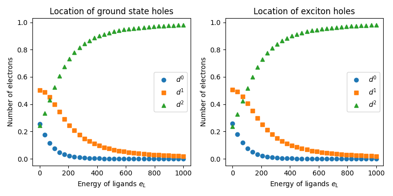
For large \(e_L\), we see that both holes are on nickel as expected. In the opposite limit of \(|e_L| \ll t\) and \(U \ll t\) the holes are shared in the ratio 0.25:0.5:0.25 as there are two ways to have one hole on Ni. In the limit of large \(e_L\), all holes move onto Ni. Since \(t\) is large, this applies equally to both the ground state and the exciton.
Connecton between atomic and charge transfer limits
We now examine the quantum numbers during cross over between the two limits with \(e_L\). Let’s first look at the how \(<S^2>\) changes for the ground state and exciton and then examine how the exciton energy changes.
U = 10
JH = 2
t = 100

eLs = np.linspace(0, 1000, 30)

info = np.array([diagonalize(U, JH, t, eL, n=6)
                 for eL in eLs])

fig, axs = plt.subplots(1, 2, figsize=(8, 4))


axs[0].plot(eLs, info[:, 4, 0], label='Ground state')
axs[0].plot(eLs, info[:, 4, 3], label='Exciton')
axs[0].set_xlabel("Energy of ligands $e_L$")
axs[0].set_ylabel('$<S^2>$')
axs[0].set_title('Quantum numbers')
axs[0].legend()

axs[1].plot(eLs, info[:, 0, 3], '+', color='C0')
axs[1].set_xlabel("Energy of ligands $e_L$")
axs[1].set_ylabel('Exciton energy', color='C0')
axr = axs[1].twinx()
axr.plot(eLs, info[:, 3, 5], 'x', color='C1')
axr.set_ylabel('$d^2$ fraction', color='C1')

for ax, color in zip([axs[1], axr], ['C0', 'C1']):
    for tick in ax.get_yticklabels():
        tick.set_color(color)

axs[1].set_ylim(0, 2*JH)
axr.set_ylim(0, 1)

axs[1].set_title('Exciton energy vs. $d^2$ character')
plt.tight_layout()
plt.show()
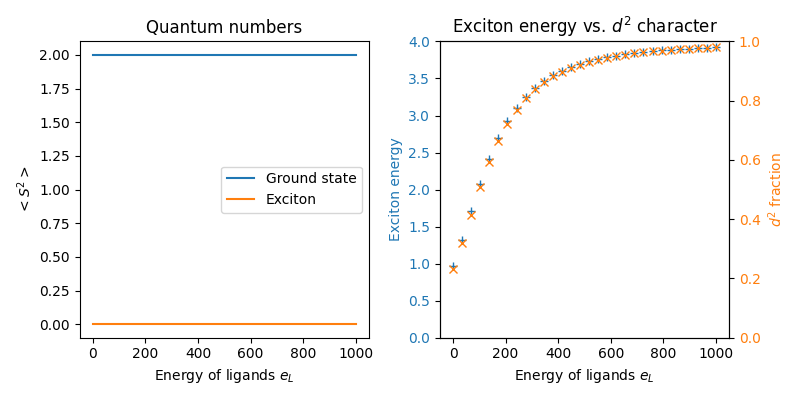
In the left panel, we see that the two limits are adiabatically connected as they preseve the same quantum numbers. This is because there is always an appreciable double occupancy under conditions where the \(d^9\underline{L}\) character is maximized and this continues to favor the high spin ground state. Other interactions such as strong tetragonal crystal field would be needed to overcome the Hund’s interactions and break this paradigm. In the right panel, we see that the exciton energy simply scales with the double occupancy. Overall, even though Hund’s interactions are irrelevant for the \(d^9\underline{L}\) electronic configuration, whenever \(t\) is appreciable there is a strong mixing with the \(d^8\) component is always present, which dominates the energy of the exciton.
Charge transfer excitons
Another limiting case of the model is where \(t\) is smaller than the Coulomb interactions. This, however, tends to produce ground state and exciton configurations that correspond to those of distinct atomic models. Let’s look at the \(e_L\) dependence in this case.
U = 10
JH = 2
t = .5
eL = 7

eLs = np.linspace(0, 20, 30)

fig, axs = plt.subplots(1, 2, figsize=(8, 4))

for ax, ind in zip(axs.ravel(), [0, 3]):
    ds = np.array([diagonalize(U, JH, t, eL, n=6)
                   for eL in eLs])

    ax.plot(eLs, ds[:, 1, ind], 'o', label='$d^0$')
    ax.plot(eLs, ds[:, 2, ind], 's', label='$d^1$')
    ax.plot(eLs, ds[:, 3, ind], '^', label='$d^2$')
    ax.set_xlabel("Energy of ligands $e_L$")
    ax.set_ylabel("Number of electrons")
    ax.legend()

axs[0].axvline(x=eL, linestyle=':', color='k')
axs[1].axvline(x=eL, linestyle=':', color='k')

axs[0].set_title("Location of ground state holes")
axs[1].set_title("Location of exciton holes")

plt.tight_layout()
plt.show()
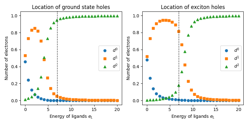
Around \(e_L = 7\) the plot shows that the excition is primairly a \(d^2 \rightarrow d^1\) transition or a \(d^8 \rightarrow d^{9}\underline{L}\) transition in electron language. Let’s examine the energy and quantum numbers.
e, d0, d1, d2, S_squared_exp, S_z_exp = diagonalize(U, JH, t, eL, n=6)

print("Ground state\nE\t<S(S+1)\tSz>")
for i in range(3):
    print(f"{e[i]:.2f}\t{S_squared_exp[i]:.2f}\t{S_z_exp[i]:.2f}")

print("\nExcited state\nE\t<S(S+1)\tSz>")
for i in range(3, 6):
    print(f"{e[i]:.2f}\t{S_squared_exp[i]:.2f}\t{S_z_exp[i]:.2f}")
Ground state
E       <S(S+1) Sz>
0.00    2.00    -1.00
0.00    2.00    -0.00
0.00    2.00    1.00

Excited state
E       <S(S+1) Sz>
2.74    0.00    0.00
2.74    0.00    0.00
2.99    0.00    0.00
We once again see the same quantum numbers, despite the differences in mixing in the ground state and exciton.
Footnotes
Total running time of the script: (0 minutes 1.206 seconds)