Exact diagonalization

Here we show how to find the eigenvalues and eigenvectors of a many-body Hamiltonian of fermions with Coulomb interactions. We then determine their spin and orbital angular momentum and how this changes when we switch on spin-orbit coupling.

Import the necessary modules.

import numpy as np
import matplotlib.pyplot as plt
import scipy
import edrixs

Parameters

Define the orbital angular momentum number $l=1$ (i.e. a p shell), the number of spin-orbitals, the occupancy and the Slater integrals. $F^k$ with $k=0,2$:

l = 1
norb = 6
noccu = 2
F0, F2 = 4.0, 1.0

Coulomb interactions

The Coulomb interactions in EDRIXS are described by a tensor. Understanding this in full is complicated and requires careful consideration of the symmetry of the interactions. See example 6 for more discussion if desired. EDRIXS can construct the matrix via

umat = edrixs.get_umat_slater('p', F0, F2)

Create basis

Now we build the binary form of the Fock basis $|F>$ (we consider it preferable to use the standard $F$ and trust the reader to avoid confusing it with the interaction parameters.) The Fock basis is the simplest legitimate form for the basis and it consists of a series of 1s and 0s where 1 means occupied and 0 means empty. These are in order up, down, up, down, up, down.

basis = edrixs.get_fock_bin_by_N(norb, noccu)
print(np.array(basis))

[[1 1 0 0 0 0]
 [1 0 1 0 0 0]
 [1 0 0 1 0 0]
 [1 0 0 0 1 0]
 [1 0 0 0 0 1]
 [0 1 1 0 0 0]
 [0 1 0 1 0 0]
 [0 1 0 0 1 0]
 [0 1 0 0 0 1]
 [0 0 1 1 0 0]
 [0 0 1 0 1 0]
 [0 0 1 0 0 1]
 [0 0 0 1 1 0]
 [0 0 0 1 0 1]
 [0 0 0 0 1 1]]

We expect the number of these states to be given by the mathematical combination of two electrons distributed among six states (three spin-orbitals with two spins per orbital).

message = ("We predict C(norb={}, noccu={})={:.0f} states and we got {:d}, "
           "which is reassuring!")
print(message.format(norb, noccu, edrixs.combination(norb, noccu), len(basis)))

We predict C(norb=6, noccu=2)=15 states and we got 15, which is reassuring!

Note that in more complicated problems with both valence and core electrons, the edrixs convention is to list the valence electrons first.

Transform interactions into Fock basis

edrixs works by initiailly creating a Hamiltonian matrix $\hat{H}$ in the single particle basis and then transforming into our chosen Fock basis. In the single particle basis, we have four fermion interactions with this form

$$\hat{H}=<F_l|\sum _{ij}{U}_{ijkl}{\hat{f}}_i^{†}{\hat{f}}_j^{†}{\hat{f}}_k{\hat{f}}_l|F_r>$$

generated as

n_fermion = 4
H = edrixs.build_opers(n_fermion, umat, basis)

We needed to specify n_fermion = 4 because the edrixs.build_opers function can also make two fermion terms.

Diagonalize the matrix

For a small problem such as this it is convenient to use the native scipy diagonalization routine. This returns eigenvalues e and eignvectors v where eigenvalue e[i] corresponds to eigenvector v[:,i].

e, v = scipy.linalg.eigh(H)
print("{} eignvalues and {} eigvenvectors {} elements long.".format(len(e),
                                                                    v.shape[1],
                                                                    v.shape[0]))

15 eignvalues and 15 eigvenvectors 15 elements long.

Computing expectation values

To interpret the results, it is informative to compute the expectations values related to the spin $\mathbf{S}$, orbital $\mathbf{L}$, and total $\mathbf{J}$, angular momentum. We first load the relevant matrices for these quantities for a p atomic shell. We need to specify that we would like to include spin when loading the orbital operator.

orb_mom = edrixs.get_orb_momentum(l, ispin=True)
spin_mom = edrixs.get_spin_momentum(l)
tot_mom = orb_mom + spin_mom

We again transform these matrices to our Fock basis to build the operators

n_fermion = 2
opL, opS, opJ = edrixs.build_opers(n_fermion, [orb_mom, spin_mom, tot_mom],
                                   basis)

Recall that quantum mechanics forbids us from knowing all three Cartesian components of angular momentum at once, so we want to compute the squares of these operators i.e.

$$\begin{array}{r}{\mathbf{S}}^2=S_x^2+S_y^2+S_z^2\\ {\mathbf{L}}^2=L_x^2+L_y^2+L_z^2\\ {\mathbf{J}}^2=J_x^2+J_y^2+J_z^2\end{array}$$

L2 = np.dot(opL[0], opL[0]) + np.dot(opL[1], opL[1]) + np.dot(opL[2], opL[2])
S2 = np.dot(opS[0], opS[0]) + np.dot(opS[1], opS[1]) + np.dot(opS[2], opS[2])
J2 = np.dot(opJ[0], opJ[0]) + np.dot(opJ[1], opJ[1]) + np.dot(opJ[2], opJ[2])

Remember that the eigenvalues of ${\mathbf{S}}^2$ are in the form $S(S+1)$ etc. and that they can be obtained by calculating the projection of the operators onto our eigenvectors.

L2_val = edrixs.cb_op(L2, v).diagonal().real
S2_val = edrixs.cb_op(S2, v).diagonal().real
J2_val = edrixs.cb_op(J2, v).diagonal().real

We can determine the degeneracy of the eigenvalues numerically and print out the values as follows

e = np.round(e, decimals=6)
degeneracy = [sum(eval == e) for eval in e]
header = "{:<3s}\t{:>8s}\t{:>8s}\t{:>8s}\t{:>8s}"
print(header.format("#  ", "E  ", "S(S+1)", "L(L+1)", "Degen."))
for i, eigenvalue in enumerate(e):
    values_list = [i, eigenvalue, S2_val[i], L2_val[i], degeneracy[i]]
    print("{:<3d}\t{:8.3f}\t{:8.3f}\t{:8.3f}\t{:>3d}".format(*values_list))

#            E            S(S+1)          L(L+1)          Degen.
0          3.800           2.000           2.000          9
1          3.800           2.000           2.000          9
2          3.800           2.000           2.000          9
3          3.800           2.000           2.000          9
4          3.800           2.000           2.000          9
5          3.800           2.000           2.000          9
6          3.800           2.000           2.000          9
7          3.800           2.000           2.000          9
8          3.800           2.000           2.000          9
9          4.040           0.000           6.000          5
10         4.040           0.000           6.000          5
11         4.040           0.000           6.000          5
12         4.040           0.000           6.000          5
13         4.040           0.000           6.000          5
14         4.400           0.000          -0.000          1

We see $S=0$ and $S=1$ states coming from the two combinations of the spin 1/2 particles. $L$ can take values of 0, 1, 2. Remember that spin states have degeneracy of $2S+1$ and the same is true for orbital states. We must multiply these $S$ and $L$ degeneracies to get the total degeneracy. Since these particles are fermions, the overall state must be antisymmetric, which dictates the allowed combinations of $S$ and $L$.

Energy level diagram

Let us show our findings graphically

fig, ax = plt.subplots()
for i, eigenvalue in enumerate(np.unique(e)):
    art = ax.plot([0, 1], [eigenvalue, eigenvalue], '-',  color='C{}'.format(i))
    ind = np.where(eigenvalue == e)[0][0]
    L = (-1 + np.sqrt(1 + 4*L2_val[ind]))/2
    S = (-1 + np.sqrt(1 + 4*S2_val[ind]))/2
    message = "L={:.0f}, S={:.0f} ({:.0f})"
    ax.text(1, eigenvalue, message.format(L, S, degeneracy[ind]),
            horizontalalignment='right',
            verticalalignment='bottom',
            color='C{}'.format(i))

ax.set_ylabel('Energy')
for loc in ['right', 'top', 'bottom']:
    ax.spines[loc].set_visible(False)

ax.yaxis.set_ticks_position('left')
ax.set_xticks([])
plt.show()

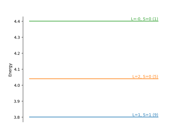
We see Hund’s rules in action! Rule 1 says that the highest spin $S=1$ state has the lowest energy. Of the two $S=0$ states, the state with larger $L=1$ is lower energy following rule 2.

Spin orbit coupling

For fun, we can see how this changes when we add spin orbit coupling (SOC). This is a two-fermion operator that we create, transform into the Fock basis and add to the prior Hamiltonian. To make things easy, let us make the SOC small so that the LS coupling approximation is valid and we can still track the states.

soc = edrixs.atom_hsoc('p', 0.1)
n_fermion = 2
H2 = H + edrixs.build_opers(n_fermion, soc, basis)

Then, we redo the diagonalization and print the results.

e2, v2 = scipy.linalg.eigh(H2)
e2 = np.round(e2, decimals=6)
degeneracy2 = [sum(eval == e2) for eval in e2]
print()
message = "With SOC\n {:<3s}\t{:>8s}\t{:>8s}\t{:>8s}\t{:>8s}\t{:>8s}"
print(message.format("#", "E", "S(S+1)", "L(L+1)", "J(J+1)", "degen."))
J2_val_soc = edrixs.cb_op(J2, v2).diagonal().real
L2_val_soc = edrixs.cb_op(L2, v2).diagonal().real
S2_val_soc = edrixs.cb_op(S2, v2).diagonal().real
for i, eigenvalue in enumerate(e2):
    values_list = [i, eigenvalue, S2_val_soc[i], L2_val_soc[i], J2_val_soc[i],
                   degeneracy2[i]]
    print("{:<3d}\t{:8.3f}\t{:8.3f}\t{:8.3f}\t{:8.3f}\t{:8.3f}".format(*values_list))

With SOC
 #             E          S(S+1)          L(L+1)          J(J+1)          degen.
0          3.673           1.927           1.927          -0.000           1.000
1          3.750           2.000           2.000           2.000           3.000
2          3.750           2.000           2.000           2.000           3.000
3          3.750           2.000           2.000           2.000           3.000
4          3.827           1.802           2.396           6.000           5.000
5          3.827           1.802           2.396           6.000           5.000
6          3.827           1.802           2.396           6.000           5.000
7          3.827           1.802           2.396           6.000           5.000
8          3.827           1.802           2.396           6.000           5.000
9          4.063           0.198           5.604           6.000           5.000
10         4.063           0.198           5.604           6.000           5.000
11         4.063           0.198           5.604           6.000           5.000
12         4.063           0.198           5.604           6.000           5.000
13         4.063           0.198           5.604           6.000           5.000
14         4.427           0.073           0.073          -0.000           1.000

and we make an equivalent energy level diagram.

fig, ax = plt.subplots()
for i, eigenvalue in enumerate(np.unique(e2)):
    art = ax.plot([0, 1], [eigenvalue, eigenvalue], '-',  color='C{}'.format(i))
    ind = np.where(eigenvalue == e2)[0][0]
    J = (-1 + np.sqrt(1+4*J2_val_soc[ind]))/2
    message = "J={:.0f} ({:.0f})"
    ax.text(1, eigenvalue, message.format(J, degeneracy2[ind]),
            horizontalalignment='right',
            verticalalignment='bottom',
            color='C{}'.format(i))

ax.set_ylabel('Energy')
for loc in ['right', 'top', 'bottom']:
    ax.spines[loc].set_visible(False)

ax.yaxis.set_ticks_position('left')
ax.set_xticks([])
plt.show()

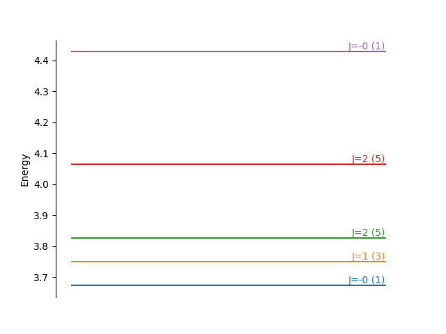
It is clear that we have split the $S=1$ state, which branches into three states from $J=|L-S|,|L-S|+1,...,|L+S|$. Since the shell is less than half full, Hund’s third rule dictates that the smaller $J$ states have the lower energies.