RIXS calculations for an atomic model¶

Here we show how to compute RIXS for a single site atomic model with crystal field and electron-electron interactions. We take the case of Sr₂YIrO₆ from Ref. [1] as the material in question. The aim of this example is to illustrate the proceedure and to provide what we hope is useful advice. What is written is not meant to be a replacement for reading the docstrings of the functions, which can always be accessed on the edrixs website or by executing functions with ?? in IPython.

import edrixs
import numpy as np
import matplotlib.pyplot as plt

Specify active core and valence orbitals¶

Sr₂YIrO₆ has a \(5d^4\) electronic configuration and we want to calculate the \(L_3\) edge spectrum i.e. resonating with a \(2p_{3/2}\) core hole. We will start by including only the \(t_{2g}\) valance orbitals.

shell_name = ('t2g', 'p32')
v_noccu = 4

Slater parameters¶

Here we want to use Hund’s interaction \(J_H\) and spin orbit coupling \(\lambda\) as adjustable parameters to match experiment. We will take the core hole interaction parameter from the Hartree Fock numbers EDRIXS has in its database. These need to be converted and arranged into the order required by EDRIXS.

Ud = 2
JH = 0.25
lam = 0.42
F0_d, F2_d, F4_d = edrixs.UdJH_to_F0F2F4(Ud, JH)
info = edrixs.utils.get_atom_data('Ir', '5d', v_noccu, edge='L3')
G1_dp = info['slater_n'][5][1]
G3_dp = info['slater_n'][6][1]
F0_dp = edrixs.get_F0('dp', G1_dp, G3_dp)
F2_dp = info['slater_n'][4][1]

slater_i = [F0_d, F2_d, F4_d]   # Fk for d
slater_n = [
    F0_d, F2_d, F4_d,   # Fk for d
    F0_dp, F2_dp,        # Fk for dp
    G1_dp, G3_dp,        # Gk for dp
    0.0, 0.0           # Fk for p
]
slater = [slater_i, slater_n]
v_soc = (lam, lam)

Diagonalization¶

We obtain the ground and intermediate state eigenenergies and the transition operators via matrix diagonalization. Note that the calculation does not know the core hole energy, so we need to adjust the energy that the resonance will appear at by hand. We know empirically that the resonance is at 11215 eV and that putting four electrons into the valance band costs about \(4 F^0_d\approx6\) eV. In this case we are assuming a perfectly cubic crystal field, which we have already implemented when we specified the use of the \(t_{2g}\) subshell only so we do not need to pass an additional v_cfmat matrix.

off = 11215 - 6
out = edrixs.ed_1v1c_py(shell_name, shell_level=(0, -off), v_soc=v_soc,
                        c_soc=info['c_soc'], v_noccu=v_noccu, slater=slater)
eval_i, eval_n, trans_op = out

edrixs >>> Running ED ...

    Summary of Slater integrals:
    ------------------------------
    Terms,   Initial Hamiltonian,  Intermediate Hamiltonian
     F0_vv :          2.0000000000        2.0000000000
     F2_vv :          2.1538461538        2.1538461538
     F4_vv :          1.3461538462        1.3461538462
     F0_vc :          0.0000000000        0.0881857143
     F2_vc :          0.0000000000        1.0700000000
     G1_vc :          0.0000000000        0.9570000000
     G3_vc :          0.0000000000        0.5690000000
     F0_cc :          0.0000000000        0.0000000000
     F2_cc :          0.0000000000        0.0000000000

edrixs >>> Dimension of the initial Hamiltonian:  15
edrixs >>> Dimension of the intermediate Hamiltonian:  24
edrixs >>> Building Many-body Hamiltonians ...
edrixs >>> Done !
edrixs >>> Exact Diagonalization of Hamiltonians ...
edrixs >>> Done !
edrixs >>> ED Done !

Compute XAS¶

To calculate XAS we need to correctly specify the orientation of the x-rays with respect to the sample. By default, the \(x, y, z\) coordinates of the sample’s crystal field, will be aligned with our lab frame, passing loc_axis to ed_1v1c_py can be used to specify a different convention. The experimental geometry is specified following the angles shown in Figure 1 of Y. Wang et al., Computer Physics Communications 243, 151-165 (2019). The default setting has x-rays along \(z\) for \(\theta=\pi/2\) rad and the x-ray beam along \(-x\) for \(\theta=\phi=0\). Parameter scatter_axis can be passed to xas_1v1c_py to specify a different geometry if desired.

Variable pol_type specifies a list of different x-ray polarizations to calculate. Here we will use so-called \(\pi\)-polarization where the x-rays are parallel to the plane spanned by the incident beam and the sample \(z\)-axis.

EDRIXS represents the system’s ground state using a set of low energy eigenstates weighted by Boltzmann thermal factors. These eigenstates are specified by gs_list, which is of the form \([0, 1, 2, 3, \dots]\). In this example, we calculate these states as those that have non-negligible thermal population. The function xas_1v1c_py assumes that the spectral broadening is dominated by the inverse core hole lifetime gamma_c, which is the Lorentzian half width at half maximum.

ominc = np.linspace(11200, 11230, 50)
temperature = 300  # in K
prob = edrixs.boltz_dist(eval_i, temperature)
gs_list = [n for n, prob in enumerate(prob) if prob > 1e-6]

thin = 30*np.pi/180
phi = 0
pol_type = [('linear', 0)]

xas = edrixs.xas_1v1c_py(
    eval_i, eval_n, trans_op, ominc, gamma_c=info['gamma_c'],
    thin=thin, phi=phi, pol_type=pol_type,
    gs_list=gs_list)

edrixs >>> Running XAS ...
edrixs >>> XAS Done !

Compute RIXS¶

Calculating RIXS is overall similar to XAS, but with a few additional considerations. The spectral width in the energy loss axis of RIXS it not set by the core hole lifetime, but by either the final state lifetime or the experimental resolution and is parameterized by gamma_f – the Lorentzian half width at half maximum.

The angle and polarization of the emitted beam must also be specified, so we pass pol_type_rixs to the function, which specifies the includes the incoming and outgoing x-ray states. If, as is common in experiments, the emitted polarization is not resolved one needs to add both emitted polarization channels, which is what we will do later on in this example.

eloss = np.linspace(-.5, 6, 400)
pol_type_rixs = [('linear', 0, 'linear', 0), ('linear', 0, 'linear', np.pi/2)]

thout = 60*np.pi/180
gamma_f = 0.02

rixs = edrixs.rixs_1v1c_py(
    eval_i, eval_n, trans_op, ominc, eloss,
    gamma_c=info['gamma_c'], gamma_f=gamma_f,
    thin=thin, thout=thout, phi=phi,
    pol_type=pol_type_rixs, gs_list=gs_list,
    temperature=temperature
)

edrixs >>> Running RIXS ...
edrixs >>> RIXS Done !

The array xas will have shape (len(ominc_xas), len(pol_type))

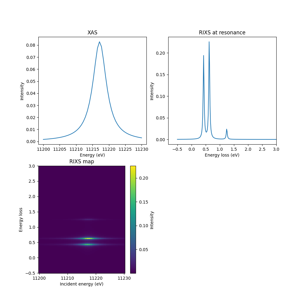
Plot XAS and RIXS¶

Let’s plot everything. We will use a function so we can reuse the code later. Note that the rixs array rixs has shape (len(ominc_xas), len(ominc_xas), len(pol_type)). We will use some numpy tricks to sum over the two different emitted polarizations.

fig, axs = plt.subplots(2, 2, figsize=(10, 10))


def plot_it(axs, ominc, xas, eloss, rixscut, rixsmap=None, label=None):
    axs[0].plot(ominc, xas[:, 0], label=label)
    axs[0].set_xlabel('Energy (eV)')
    axs[0].set_ylabel('Intensity')
    axs[0].set_title('XAS')

    axs[1].plot(eloss, rixscut, label=f"{label}")
    axs[1].set_xlabel('Energy loss (eV)')
    axs[1].set_ylabel('Intensity')
    axs[1].set_title(f'RIXS at resonance')

    if rixsmap is not None:
        art = axs[2].pcolormesh(ominc, eloss, rixsmap.T, shading='auto')
        plt.colorbar(art, ax=axs[2], label='Intensity')
        axs[2].set_xlabel('Incident energy (eV)')
        axs[2].set_ylabel('Energy loss')
        axs[2].set_title('RIXS map')


rixs_pol_sum = rixs.sum(-1)
cut_index = np.argmax(rixs_pol_sum[:, eloss < 2].sum(1))
rixscut = rixs_pol_sum[cut_index]

plot_it(axs.ravel(), ominc, xas, eloss, rixscut, rixsmap=rixs_pol_sum)
axs[0, 1].set_xlim(right=3)
axs[1, 0].set_ylim(top=3)
axs[1, 1].remove()

plt.show()

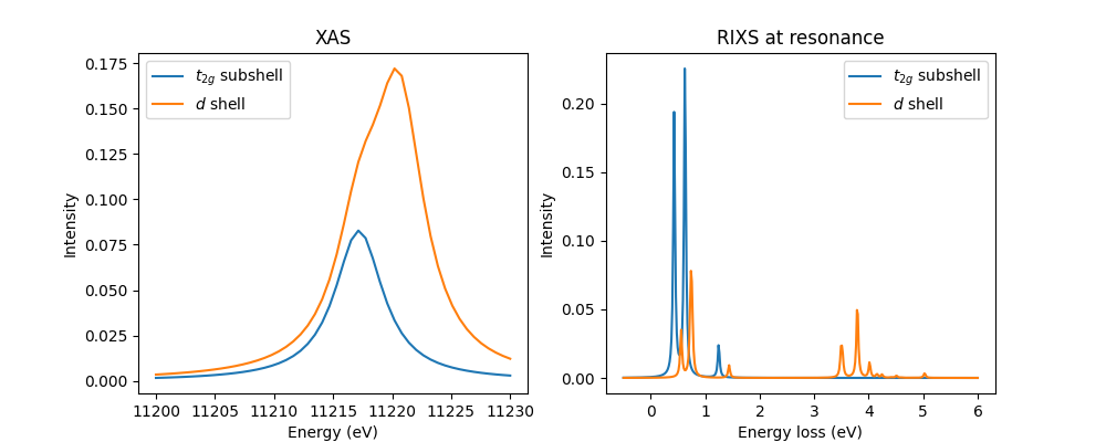
Full d shell calculation¶

Some researchers have questioned the appropriateness of only including the \(t_{2g}\) subshell for iridates [2]. Let’s test this. We specify that the full \(d\) shell should be used and apply cubic crystal field matrix v_cfmat. We shift the energy offset by \(\frac{2}{5}10D_q\), which is the amount the crystal field moves the \(t_{2g}\) subshell.

ten_dq = 3.5
v_cfmat = edrixs.cf_cubic_d(ten_dq)
off = 11215 - 6 + ten_dq*2/5
out = edrixs.ed_1v1c_py(('d', 'p32'), shell_level=(0, -off), v_soc=v_soc,
                        v_cfmat=v_cfmat,
                        c_soc=info['c_soc'], v_noccu=v_noccu, slater=slater)
eval_i, eval_n, trans_op = out

xas_full_d_shell = edrixs.xas_1v1c_py(
    eval_i, eval_n, trans_op, ominc, gamma_c=info['gamma_c'],
    thin=thin, phi=phi, pol_type=pol_type,
    gs_list=gs_list)

rixs_full_d_shell = edrixs.rixs_1v1c_py(
    eval_i, eval_n, trans_op, np.array([11215]), eloss,
    gamma_c=info['gamma_c'], gamma_f=gamma_f,
    thin=thin, thout=thout, phi=phi,
    pol_type=pol_type_rixs, gs_list=gs_list,
    temperature=temperature)

fig, axs = plt.subplots(1, 2, figsize=(10, 4))
plot_it(axs, ominc, xas, eloss, rixscut, label='$t_{2g}$ subshell')
rixscut = rixs_full_d_shell.sum((0, -1))
plot_it(axs, ominc, xas_full_d_shell, eloss, rixscut, label='$d$ shell')

axs[0].legend()
axs[1].legend()
plt.show()

edrixs >>> Running ED ...

    Summary of Slater integrals:
    ------------------------------
    Terms,   Initial Hamiltonian,  Intermediate Hamiltonian
     F0_vv :          2.0000000000        2.0000000000
     F2_vv :          2.1538461538        2.1538461538
     F4_vv :          1.3461538462        1.3461538462
     F0_vc :          0.0000000000        0.0881857143
     F2_vc :          0.0000000000        1.0700000000
     G1_vc :          0.0000000000        0.9570000000
     G3_vc :          0.0000000000        0.5690000000
     F0_cc :          0.0000000000        0.0000000000
     F2_cc :          0.0000000000        0.0000000000

edrixs >>> Dimension of the initial Hamiltonian:  210
edrixs >>> Dimension of the intermediate Hamiltonian:  1008
edrixs >>> Building Many-body Hamiltonians ...
edrixs >>> Done !
edrixs >>> Exact Diagonalization of Hamiltonians ...
edrixs >>> Done !
edrixs >>> ED Done !
edrixs >>> Running XAS ...
edrixs >>> XAS Done !
edrixs >>> Running RIXS ...
edrixs >>> RIXS Done !

As expected, we see the appearance of excitations on the energy scale of \(10D_q\) in the XAS and RIXS. The low energy manifold is qualitatively, but not quantiatively similar. This makes it clear that the parameterization of Sr₂YIrO₆ is dependent on the model.

Footnotes

Total running time of the script: (0 minutes 4.640 seconds)

Gallery generated by Sphinx-Gallery