Note
Go to the end to download the full example code.
Hubbard Dimer
This exercise will demonstrate how to handle hopping and multi-site problems within edrixs using the example of a Hubbard dimer. We want to solve the equation
\[\begin{equation} \hat{H} = \sum_{i,j} \sum_{\sigma} t_{i,j} \hat{f}^{\dagger}_{i,\sigma} \hat{f}_{j, \sigma} + U \sum_{i} \hat{n}_{i,\uparrow}\hat{n}_{i,\downarrow}, \end{equation}\]
which involves two sites labeled with indices \(i\) or \(j\) with two electrons of spin \(\sigma\in{\uparrow,\downarrow}\). \(t_{i,j}\) is the hopping between sites, \(\hat{f}^{\dagger}_{i,\sigma}\) is the creation operators, and \(\hat{n}^{\dagger}_{i,\sigma}=\hat{f}^{\dagger}_{i,\sigma}\hat{f}_{i,\sigma}\) is the number operator. The main task is to represent this Hamiltonian and the related spin operator using the EDRIXS two-fermion and four-fermion form where \(\alpha,\beta,\delta,\gamma\) are the indices of the single particle basis.
\[\begin{equation} \hat{H} = \sum_{\alpha,\beta} t_{\alpha,\beta} \hat{f}^{\dagger}_{\alpha} \hat{f}_{\beta} + \sum_{\alpha,\beta,\gamma,\delta} U_{\alpha,\beta,\gamma,\delta} \hat{f}^{\dagger}_{\alpha}\hat{f}^{\dagger}_{\beta}\hat{f}_{\gamma}\hat{f}_{\delta}. \end{equation}\]
Initialize matrices
We start by noting that each of the two sites is like an \(l=0\) \(s\)-orbital with two spin-orbitals each. We will include two electron occupation and build the Fock basis.
Create function to populate and diagonalize matrices
The Coulomb and hopping matrices umat and emat will be
represented by \(4\times4\times4\times4\) and \(4\times4\) matrices,
respectively. Note that we needed to specify
that these are, in general, complex, although
they happen to contain only real numbers in this case. We follow the convention
that these are ordered first by site and then by spin:
\(|0\uparrow>, |0\downarrow>, |1\uparrow>, |1\downarrow>\).
Consequently the \(2\times2\) and \(2\times2\times2\times2\) block
diagonal structures of the matrices will contain the on-site interactions.
The converse is true for the hopping between the sites.
From here let us generate a function to build and diagonalize the Hamiltonian.
We need to generate the Coulomb matrix for the on-site interactions and
apply it to the block diagonal. The hopping connects off-site indices with
the same spin.
def diagonalize(U, t, extra_emat=None):
    """Diagonalize 2 site Hubbard Hamiltonian"""
    umat = np.zeros((norb, norb, norb, norb), dtype=np.complex128)
    emat = np.zeros((norb, norb), dtype=np.complex128)
    U_mat_1site = edrixs.get_umat_slater('s', U)
    umat[:2, :2, :2, :2,] = umat[2:, 2:, 2:, 2:] = U_mat_1site
    emat[2, 0] = emat[3, 1] = emat[0, 2] = emat[1, 3] = t

    if extra_emat is not None:
        emat = emat + extra_emat

    H = (edrixs.build_opers(2, emat, basis)
         + edrixs.build_opers(4, umat, basis))

    e, v = scipy.linalg.eigh(H)
    return e, v
The large \(U\) limit
Let us see what happens with \(U \gg t\).
Energies are
[  -0.004    0.       0.       0.    1000.    1000.004]
To analyze what is going on we can determine the spin expectation values of the cluster. Building the operators follows the same form as the Hamiltonian and the previous example.
spin_mom_one_site = edrixs.get_spin_momentum(ll)
spin_mom = np.zeros((3, norb, norb), dtype=np.complex128)
spin_mom[:, :2, :2] = spin_mom[:, 2:, 2:] = spin_mom_one_site

opS = edrixs.build_opers(2, spin_mom, basis)
opS_squared = (np.dot(opS[0], opS[0]) + np.dot(opS[1], opS[1])
               + np.dot(opS[2], opS[2]))
This time let us include a tiny magnetic field along the \(z\)-axis, so that we have a well-defined measurement axis and print out the expectation values.
zeeman = np.zeros((norb, norb), dtype=np.complex128)
zeeman[:2, :2] = zeeman[2:, 2:] = 1e-8*spin_mom_one_site[2]
e, v = diagonalize(1000, 1, extra_emat=zeeman)

Ssq_exp = edrixs.cb_op(opS_squared, v).diagonal().real
Sz_exp = edrixs.cb_op(opS[2], v).diagonal().real

header = "{:<10s}\t{:<6s}\t{:<6s}"
print(header.format("E", "S(S+1)", "<Sz>"))
for i in range(len(e)):
    print("{:<2f}\t{:.1f}\t{:.1f}".format(e[i], Ssq_exp[i], Sz_exp[i]))
E               S(S+1)  <Sz>
-0.004000       0.0     0.0
-0.000000       2.0     -1.0
-0.000000       2.0     0.0
0.000000        2.0     1.0
1000.000000     0.0     0.0
1000.004000     0.0     0.0
For \(U \gg t\) the two states with double occupancy acquire an energy of approximately \(U\). The low energy states are a \(S=0\) singlet and and \(S=1\) triplet, which are split by \(4t^2/U\), which is the magnetic exchange term.
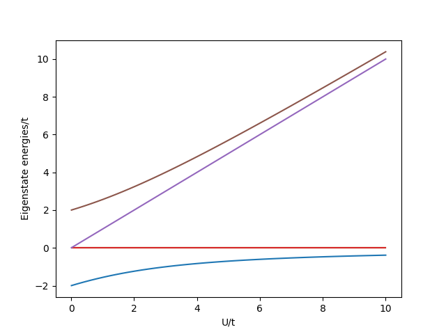
\(U\) dependence
Let us plot the changes in energy with \(U\).
plt.figure()

t = 1
Us = np.linspace(0.01, 10, 50)
Es = np.array([diagonalize(U, t, extra_emat=zeeman)[0] for U in Us])

plt.plot(Us/t, Es/t)
plt.xlabel('U/t')
plt.ylabel('Eigenstate energies/t')
plt.show()
To help interpret this, we can represent the eigenvectors in terms of a sum of the single particle states.
def get_single_particle_repesentations(v):
    reps = []
    for i in range(6):
        rep = sum([vec*weight for weight, vec
                        in zip(v[:, i], np.array(basis))])
        reps.append(rep)

    return np.array(reps)

t = 1
for U in [10000, 0.0001]:
    e, v = diagonalize(U, t, extra_emat=zeeman)
    repesentations = get_single_particle_repesentations(v)
    print("For U={} t={} states  are".format(U,  t))
    print(repesentations.round(3).real)
    print("\n")
For U=10000 t=1 states  are
[[-0.707  0.707  0.707 -0.707]
 [ 0.     1.     0.     1.   ]
 [ 0.707  0.707  0.707  0.707]
 [-1.     0.    -1.     0.   ]
 [-0.707 -0.707  0.707  0.707]
 [ 0.707  0.707  0.707  0.707]]


For U=0.0001 t=1 states  are
[[-0.     1.     1.    -0.   ]
 [ 0.     1.     0.     1.   ]
 [ 0.707  0.707  0.707  0.707]
 [-1.     0.    -1.     0.   ]
 [-0.707 -0.707  0.707  0.707]
 [-1.    -0.    -0.    -1.   ]]
For \(U \gg t\) the ground state maximizes its magnetic exchange energy saving. In the \(U \ll t\) condition the ground state maximizes its kinetic energy saving. Since both states share the same parity, the cross-over between them is smooth. This type of physics is at play in current research on quantum materials [1] [2].
Footnotes
Total running time of the script: (0 minutes 0.095 seconds)