Ground state analysis for NiO

This example follows the Anderson impurity model for NiO XAS example and considers the same model. This time we show how to analyze the wavevectors in terms of a \(\alpha |d^8L^{10}> + \beta |d^9L^9> \gamma |d^{10}L^8>\) representation.

In doing this we will go through the exercise of building and diagonalizing the Hamiltonian in a way that hopefully clarifies how to analyze other properties of the model.

import edrixs
import numpy as np
import matplotlib.pyplot as plt
import scipy
import example_3_AIM_XAS
import importlib
_ = importlib.reload(example_3_AIM_XAS)

Hamiltonian

edrixs builds model Hamiltonians based on two fermion and four fermion terms. The four fermion terms come from Coulomb interactions and will be assigned to umat. All other interactions contribute to two fermion terms in emat.

\[\begin{equation} \hat{H}_{i} = \sum_{\alpha,\beta} t_{\alpha,\beta} \hat{f}^{\dagger}_{\alpha} \hat{f}_{\beta} + \sum_{\alpha,\beta,\gamma,\delta} U_{\alpha,\beta,\gamma,\delta} \hat{f}^{\dagger}_{\alpha}\hat{f}^{\dagger}_{\beta} \hat{f}_{\gamma}\hat{f}_{\delta}, \end{equation}\]

Import parameters

Let’s get the parammeters we need from the Anderson impurity model for NiO XAS example. We need to consider ntot=20 spin-orbitals for this problem.

from example_3_AIM_XAS import (F0_dd, F2_dd, F4_dd,
                               nd, norb_d, norb_bath, v_noccu,
                               imp_mat, CF, bath_level,
                               hyb, ext_B, trans_c2n)
ntot = 20

Four fermion matrix

The Coulomb interactions in the \(d\) shell of this problem are described by a \(10\times10\times10\times10\) matrix. We need to specify a \(20\times20\times20\times 20\) matrix since we need to include the full problem with ntot=20 spin-orbitals. The edrixs convention is to put the \(d\) orbitals first, so we assign them to the first \(10\times10\times10\times 10\) indices of the matrix. edrixs creates this matrix in the complex harmmonic basis by default.

umat_delectrons = edrixs.get_umat_slater('d', F0_dd, F2_dd, F4_dd)
umat = np.zeros((ntot, ntot, ntot, ntot), dtype=complex)
umat[:norb_d, :norb_d, :norb_d, :norb_d] += umat_delectrons

Two fermion matrix

Previously we made a \(10\times10\) two-fermion matrix describing the \(d\)-shell interactions. Keep in mind we did this in the real harmonic basis. We need to specify the two-fermion matrix for the full problem \(20\times20\) spin-orbitals in size.

emat_rhb = np.zeros((ntot, ntot), dtype='complex')
emat_rhb[0:norb_d, 0:norb_d] += imp_mat

The bath_level energies need to be applied to the diagonal of the last \(10\times10\) region of the matrix.

indx = np.arange(norb_d, norb_d*2)
emat_rhb[indx, indx] += bath_level[0]

The hyb terms mix the impurity and bath states and are therefore applied to the off-diagonal terms of emat.

indx1  = np.arange(norb_d)
indx2 = np.arange(norb_d, norb_d*2)
emat_rhb[indx1, indx2] += hyb[0]
emat_rhb[indx2, indx1] += np.conj(hyb[0])

We now need to transform into the complex harmonic basis. We assign the two diagonal blocks of a \(20\times20\) matrix to the conjugate transpose of the transition matrix.

tmat = np.eye(ntot, dtype=complex)
for i in range(2):
    off = i * norb_d
    tmat[off:off+norb_d, off:off+norb_d] = np.conj(np.transpose(trans_c2n))

emat_chb = edrixs.cb_op(emat_rhb, tmat)

The spin exchange is built from the spin operators and the effective field is applied to the \(d\)-shell region of the matrix.

v_orbl = 2
sx = edrixs.get_sx(v_orbl)
sy = edrixs.get_sy(v_orbl)
sz = edrixs.get_sz(v_orbl)
zeeman = ext_B[0] * (2 * sx) + ext_B[1] * (2 * sy) + ext_B[2] * (2 * sz)
emat_chb[0:norb_d, 0:norb_d] += zeeman

Build the Fock basis and Hamiltonain and Diagonalize

We create the fock basis and build the Hamiltonian using the full set of \(20\) spin orbitals, specifying that they are occuplied by \(18\) electrons. See the Exact diagonalization example for more details if needed. We also set the ground state to zero energy.

basis = np.array(edrixs.get_fock_bin_by_N(ntot, v_noccu))
H = (edrixs.build_opers(2, emat_chb, basis)
  + edrixs.build_opers(4, umat, basis))

e, v = scipy.linalg.eigh(H)
e -= e[0]

State analysis

Now we have all the eigenvectors in the Fock basis, we need to pick out the states that have 8, 9 and 10 \(d\)-electrons, respectively. The modulus squared of these coeffcients need to be added up to get \(\alpha\), \(\beta\), and \(\gamma\).

num_d_electrons = basis[:, :norb_d].sum(1)

alphas = np.sum(np.abs(v[num_d_electrons==8, :])**2, axis=0)
betas = np.sum(np.abs(v[num_d_electrons==9, :])**2, axis=0)
gammas = np.sum(np.abs(v[num_d_electrons==10, :])**2, axis=0)

The ground state is the first entry.

message = "Ground state\nalpha={:.3f}\tbeta={:.3f}\tgamma={:.3f}"
print(message.format(alphas[0], betas[0], gammas[0]))

Ground state
alpha=0.825     beta=0.171      gamma=0.004

Plot

Let’s look how \(\alpha\), \(\beta\), and \(\gamma\) vary with energy.

fig, ax = plt.subplots()

ax.plot(e, alphas, label=r'$\alpha$ $d^8L^{10}$')
ax.plot(e, betas, label=r'$\beta$ $d^9L^{9}$')
ax.plot(e, gammas, label=r'$\gamma$ $d^{10}L^{8}$')

ax.set_xlabel('Energy (eV)')
ax.set_ylabel('Population')
ax.set_title('NiO')
ax.legend()
plt.show()

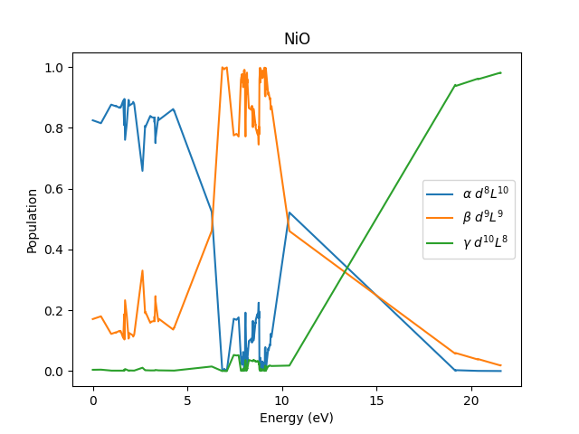
We see that the ligand states are mixed into the ground state, but the majority of the weight for the \(L^9\) and \(L^8\) states live at \(\Delta\) and \(2\Delta\). With a lot of additional structure from the other interactions.