Note
Go to the end to download the full example code.
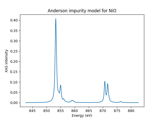
Anderson impurity model for NiO XAS
Here we calculate the \(L\)-edge XAS spectrum of an Anderson impurity model, which is sometimes also called a charge-transfer multiplet model. This model considers a set of correlated orbitals, often called the impurity or metal states, that hybridize with a set of uncorrelated orbitals, often called the ligands or bath states. Everyone’s favorite test case for x-ray spectroscopic calculations of the Anderson impurity model is NiO and we won’t risk being original! This means that our correlated states will be the Ni \(3d\) orbitals and the uncorrelated states come from O \(2p\) orbitals. The fact that we include these interactions means that our spectrum can include processes where electrons transition from the bath to the impurity, as such the Anderson Impurity Model is often more accurate than atomic models, especially if the material has strong covalency.
When defining the bath states, it is useful to use the so-called
symmetry adapted linear combinations of orbitals as the basis. These states
take into account the symmetry relationships between the different bath atom
orbitals and the fact that there are bath orbital combinations that do not
interact with the impurity by symmetry. By doing this the problem can be
represented with fewer orbitals, which makes the calculation far more efficient.
The standard EDRIXS solver that we will use assumes that the bath states are
represented by an integer number of bath sites set by nbath, each of
which hosts the same number of spin-orbits as the impurity e.g. 10 for a
\(d\)-electron material.
NiO has a rocksalt structure in which all Ni atoms are surrounded by six O atoms. This NiO cluster used to simulate the crystal would then contain 10 Ni \(3d\) spin-orbitals and \(6\) spin-orbitals per O \(\times 6\) O atoms \(=36\) oxygen spin-orbitals. As explained by, for example, Maurits Haverkort et al. in [1] symmetry allows us to represent the bath with 10 symmetry adapted linear combinations of the different O \(p_x, p_y, p_z\) states. The crystal field and hopping parameters for such a calculation can be obtained by post-processing DFT calculations. We will use values for NiO from [1]. If you use values from a paper the relevant references should, of course, be cited.
import edrixs
import numpy as np
import matplotlib.pyplot as plt
Number of electrons
When formulating problems of this type, one usually thinks of a nominal
valence for the impurity atom in this case nd = 8 and assume that the
bath is full. The solver that we will
use can simulate multiple bath sites. In our case we specify
nbath = 1 sites. Electrons will be able to transition from O to Ni
during our calculation, but the total number of valance electrons
v_noccu will be conserved.
Coulomb interactions
The atomic Coulomb interactions are usually initialized based on Hartree-Fock calculations from, for example, Cowan’s code. edrixs has a database of these.
The atomic values are typically scaled to account for screening in the solid. Here we use 80% scaling. Let’s write these out in full, so that nothing is hidden. Values for \(U_{dd}\) and \(U_{dp}\) are those of Ref. [1] obtained by comparing theory and experiment [2] [3].
scale_dd = 0.8
F2_dd = info['slater_i'][1][1] * scale_dd
F4_dd = info['slater_i'][2][1] * scale_dd
U_dd = 7.3
F0_dd = U_dd + edrixs.get_F0('d', F2_dd, F4_dd)

scale_dp = 0.8
F2_dp = info['slater_n'][4][1] * scale_dp
G1_dp = info['slater_n'][5][1] * scale_dp
G3_dp = info['slater_n'][6][1] * scale_dp
U_dp = 8.5
F0_dp = U_dp + edrixs.get_F0('dp', G1_dp, G3_dp)

slater = ([F0_dd, F2_dd, F4_dd],  # initial
          [F0_dd, F2_dd, F4_dd, F0_dp, F2_dp, G1_dp, G3_dp])  # with core hole
Energy of the bath states
In the notation used in EDRIXS, \(\Delta\) sets the energy difference
between the bath and impurity states. \(\Delta\) is defined in the atomic
limit without crystal field (i.e. in terms of the centers of the impurity and
bath states before hybridization is considered) as the energy for a
\(d^{n_d} \rightarrow d^{n_d + 1} \underline{L}\) transition.
Note that as electrons are moved one has to pay energy
costs associated with the Coulomb interactions. The
energy splitting between the bath and impurity is consequently not simply
\(\Delta\). One must therefore determine the energies by solving
a set of linear equations. See the edrixs.utils functions
for details. We can call these functions to get the impurity energy
\(E_d\), bath energy \(E_L\), impurity energy with a core hole
\(E_{dc}\), bath energy with a core hole \(E_{Lc}\) and the
core hole energy \(E_p\). The
if __name__ == '__main__' code specifies that this command
should only be executed if the file is explicitly run.
Delta = 4.7
E_d, E_L = edrixs.CT_imp_bath(U_dd, Delta, nd)
E_dc, E_Lc, E_p = edrixs.CT_imp_bath_core_hole(U_dd, U_dp, Delta, nd)
message = ("E_d = {:.3f} eV\n"
           "E_L = {:.3f} eV\n"
           "E_dc = {:.3f} eV\n"
           "E_Lc = {:.3f} eV\n"
           "E_p = {:.3f} eV\n")
if __name__ == '__main__':
    print(message.format(E_d, E_L, E_dc, E_Lc, E_p))
E_d = -41.189 eV
E_L = 12.511 eV
E_dc = -77.367 eV
E_Lc = 27.333 eV
E_p = -44.467 eV
The spin-orbit coupling for the valence electrons in the ground state, the valence electrons with the core hole present, and for the core hole itself are initialized using the atomic values.
Build matrices describing interactions
edrixs uses complex spherical harmonics as its default basis set. If we want to
use another basis set, we need to pass a matrix to the solver, which transforms
from complex spherical harmonics into the basis we use.
The solver will use this matrix when implementing the Coulomb interactions
using the slater list of Coulomb parameters.
Here it is easiest to
use real harmonics. We make the complex harmonics to real harmonics transformation
matrix via
trans_c2n = edrixs.tmat_c2r('d',True)
The crystal field and SOC needs to be passed to the solver by constructing the impurity matrix in the real harmonic basis. For cubic symmetry, we need to set the energies of the orbitals along the diagonal of the matrix. These need to be in pairs as there are two spin-orbitals for each orbital energy. Python list comprehension and numpy indexing are used here. See Crystal fields for more details if needed.
ten_dq = 0.56
CF = np.zeros((norb_d, norb_d), dtype=complex)
diagonal_indices = np.arange(norb_d)

orbital_energies = np.array([e for orbital_energy in
                             [+0.6 * ten_dq, # dz2
                              -0.4 * ten_dq, # dzx
                              -0.4 * ten_dq, # dzy
                              +0.6 * ten_dq, # dx2-y2
                              -0.4 * ten_dq] # dxy)
                             for e in [orbital_energy]*2])


CF[diagonal_indices, diagonal_indices] = orbital_energies
The valence band SOC is constructed in the normal way and transformed into the real harmonic basis.
The total impurity matrices for the ground and core-hole states are then
the sum of crystal field and spin-orbit coupling. We further needed to apply
an energy shift along the matrix diagonal, which we do using the
np.eye function which creates a diagonal matrix of ones.
The energy level of the bath(s) is described by a matrix where the row index
denotes which bath and the column index denotes which orbital. Here we have
only one bath, with 10 spin-orbitals. We initialize the matrix to
norb_d and then split the energies according to ten_dq_bath.
ten_dq_bath = 1.44
bath_level = np.full((nbath, norb_d), E_L, dtype=complex)
bath_level[0, :2] += ten_dq_bath*.6  # 3z2-r2
bath_level[0, 2:6] -= ten_dq_bath*.4  # zx/yz
bath_level[0, 6:8] += ten_dq_bath*.6  # x2-y2
bath_level[0, 8:] -= ten_dq_bath*.4  # xy
bath_level_n = np.full((nbath, norb_d), E_Lc, dtype=complex)
bath_level_n[0, :2] += ten_dq_bath*.6  # 3z2-r2
bath_level_n[0, 2:6] -= ten_dq_bath*.4  # zx/yz
bath_level_n[0, 6:8] += ten_dq_bath*.6  # x2-y2
bath_level_n[0, 8:] -= ten_dq_bath*.4  # xy
The hybridization matrix describes the hopping between the bath and the impurity. This is called either \(V\) or \(T\) in the literature and matrix sign can either be positive or negative based. This is the same shape as the bath matrix. We take our values from Maurits Haverkort et al.’s DFT calculations [1].
We now need to define the parameters describing the XAS. X-ray polarization can be linear, circular or isotropic (appropriate for a powder).
poltype_xas = [('isotropic', 0)]
edrixs uses the temperature in Kelvin to work out the population of the low-lying states via a Boltzmann distribution.
temperature = 300
The x-ray beam is specified by the incident angle and azimuthal angle in radians
these are with respect to the crystal field \(z\) and \(x\) axes
written above. (That is, unless you specify the loc_axis parameter
described in the edrixs.xas_siam_fort function documentation.)
The spectrum in the raw calculation is offset by the energy involved with the
core hole state, which is roughly \(5 E_p\), so we offset the spectrum by
this and use om_shift as an adjustable parameters for comparing
theory to experiment. We also use this to specify ominc_xas
the range we want to compute the spectrum over. The core hole lifetime
broadening also needs to be set via gamma_c_stat.
The final state broadening is specified in terms of half-width at half-maximum
You can either pass a constant value or an array the same size as
om_shift with varying values to simulate, for example, different state
lifetimes for higher energy states.
gamma_c = np.full(ominc_xas.shape, 0.48/2)
Magnetic field is a three-component vector in eV specified with respect to the
same local axis as the x-ray beam. Since we are considering a powder here
we create an isotropic normalized vector. on_which = 'both' specifies to
apply the operator to the total spin plus orbital angular momentum as is
appropriate for a physical external magnetic field. You can use
on_which = 'spin' to apply the operator to spin in order to simulate
magnetic order in the sample. The value of the Bohr Magneton can
be useful for converting here \(\mu_B = 5.7883818012\times 10^{−5}\).
For this example, we will account for magnetic order in the sample by
The number crunching uses mpi4py. You can safely ignore this for most purposes, but see Y. L. Wang et al., Computer Physics Communications 243, 151-165 (2019) if you would like more details. The main thing to remember is that you should call this script via:
mpirun -n <number of processors> python example_AIM_XAS.py
where <number of processors> is the number of processors
you’d like to us. Running it as normal will work, it will just be slower.
Calling the edrixs.ed_siam_fort solver will find the ground state and
write input files, hopping_i.in, hopping_n.in, coulomb_i.in, coulomb_n.in
for following XAS (or RIXS) calculation. We need to specify siam_type=0
which says that we will pass imp_mat, bath_level and hyb.
We need to specify do_ed = 1. For this example, we cannot use
do_ed = 0 for a ground state search as we have set the impurity and
bath energy levels artificially, which means edrixs will have trouble to know
which subspace to search to find the ground state.
if __name__ == '__main__':
    do_ed = 1
    eval_i, denmat, noccu_gs = edrixs.ed_siam_fort(
        comm, shell_name, nbath, siam_type=0, imp_mat=imp_mat, imp_mat_n=imp_mat_n,
        bath_level=bath_level, bath_level_n=bath_level_n, hyb=hyb, c_level=c_level,
        c_soc=c_soc, slater=slater, ext_B=ext_B,
        on_which=on_which, trans_c2n=trans_c2n, v_noccu=v_noccu, do_ed=do_ed,
        ed_solver=2, neval=50, nvector=3, ncv=100, idump=True)
edrixs >>> Running ED ...

    Summary of Slater integrals:
    ------------------------------
    Terms,  Initial Hamiltonian,  Intermediate Hamiltonian
     F0_vv :          7.8036698413        7.8036698413
     F2_vv :          9.7872000000        9.7872000000
     F4_vv :          6.0784000000        6.0784000000
     F0_vc :          0.0000000000        8.9214742857
     F2_vc :          0.0000000000        6.1768000000
     G1_vc :          0.0000000000        4.6296000000
     G3_vc :          0.0000000000        2.6328000000
     F0_cc :          0.0000000000        0.0000000000
     F2_cc :          0.0000000000        0.0000000000

edrixs >>> do_ed=1, perform ED at noccu:  18
Let’s check that we have all the electrons we think we have and print how the electron are distributed between the Ni (impurity) and O (bath).
if __name__ == '__main__':
    assert np.abs(noccu_gs - v_noccu) < 1e-6
    impurity_occupation = np.sum(denmat[0].diagonal()[0:norb_d]).real
    bath_occupation = np.sum(denmat[0].diagonal()[norb_d:]).real
    print('Impurity occupation = {:.6f}\n'.format(impurity_occupation))
    print('Bath occupation = {:.6f}\n'.format(bath_occupation))
Impurity occupation = 8.179506

Bath occupation = 9.820494
We see that 0.18 electrons move from the O to the Ni in the ground state.
We can now construct the XAS spectrum edrixs by applying a transition
operator to create the excited state. We need to be careful to specify how
many of the low energy states are thermally populated. In this case
num_gs=3. This can be determined by inspecting the function output.
if __name__ == '__main__':
    xas, xas_poles = edrixs.xas_siam_fort(
        comm, shell_name, nbath, ominc_xas, gamma_c=gamma_c, v_noccu=v_noccu, thin=thin,
        phi=phi, num_gs=3, nkryl=200, pol_type=poltype_xas, temperature=temperature
    )
edrixs >>> Running XAS ...
edrixs >>> Loop over for polarization:  0 isotropic
edrixs >>> Isotropic, component:  0
edrixs >>> Loop over for polarization:  0 isotropic
edrixs >>> Isotropic, component:  1
edrixs >>> Loop over for polarization:  0 isotropic
edrixs >>> Isotropic, component:  2
Let’s plot the data and save it just in case
if __name__ == '__main__':
    fig, ax = plt.subplots()

    ax.plot(ominc_xas, xas)
    ax.set_xlabel('Energy (eV)')
    ax.set_ylabel('XAS intensity')
    ax.set_title('Anderson impurity model for NiO')
    plt.show()

    np.savetxt('xas.dat', np.concatenate((np.array([ominc_xas]).T, xas), axis=1))
Footnotes
Total running time of the script: (0 minutes 0.548 seconds)