Note
Go to the end to download the full example code.
X-ray transitions
This example explains how to calculate x-ray transition amplitudes between specific orbital and spin states. We take the case of a cuprate which has one hole in the \(d_{x^2-y^2}\) orbital and a spin ordering direction along the in-plane diagaonal direction and compute the angular dependence of spin-flip and non-spin-flip processes.
This case was chosen because the eigenvectors in question are simple enough for us to write them out more-or-less by hand, so this example helps the reader to understand what happens under the hood in more complex cases.
Some of the code here is credited to Yao Shen who used this approach for the analysis of a low valence nickelate material [1]. The task performed repeats analysis done by many researchers e.g. Luuk Ament et al [2] as well as several other groups.
import edrixs
import numpy as np
import matplotlib.pyplot as plt
import scipy
Eigenvectors
Let us start by determining the eigenvectors involved in the transitions. The spin direction can be set using a vector \(\vec{B}\) to represent a magnetic field in terms of generalized spin operator \(\tilde{\sigma}=\vec{B}\cdot\sigma\) based on the Pauli matrices \(\sigma\). Let’s put the spin along the \([1, 1, 0]\) direction and formuate the problem in the hole basis. For one particle, we know that the Hamiltonian will be diagonal in the real harmonic basis. We can generate the required eigenvectors by making a diagonal matrix, transforming it to the required complex harmonic basis (as is standard for EDRIXS) and diagonalizing it. As long as the crystal field splitting is much larger than the magnetic field, the eigenvectors will be independent of the exact values of both these parameters.
B = 1e-3*np.array([1, 1, 0])
cf_splitting = 1e3
zeeman = sum(s*b for s, b in zip(edrixs.get_spin_momentum(2), B))
dd_levels = np.array([energy for dd_level in cf_splitting*np.arange(5)
                      for energy in [dd_level]*2], dtype=complex)
emat_rhb = np.diag(dd_levels)
emat = edrixs.cb_op(emat_rhb, edrixs.tmat_r2c('d', ispin=True)) + zeeman
_, eigenvectors = np.linalg.eigh(emat)

def get_eigenvector(orbital_index, spin_index):
    return eigenvectors[:, 2*orbital_index + spin_index]
Let’s examine the \(d_{x^2-y^2}\) orbital first. Recall from the
Crystal fields
example that edrixs uses the standard orbital order of
\(d_{3z^2-r^2}, d_{xz}, d_{yz}, d_{x^2-y^2}, d_{xy}\). So we want
orbital_index = 3 element. Using this, we can build spin-up and -down
eigenvectors.
orbital_index = 3

groundstate_vector = get_eigenvector(orbital_index, 0)
excitedstate_vector = get_eigenvector(orbital_index, 1)
Transition operators and scattering matrix
Here we are considering the \(L_3\)-edge. This means a \(2p_{3/2} \rightarrow 3d\) absoprtion transition and a \(2p_{3/2} \rightarrow 3d\) emission transition. We can read the relevant matrix from the edrixs database, keeping in mind that there are in fact three operations for \(x, y,\) & \(z\) directions. Note that edrixs provides operators in electron notation. If we define \(D\) as the transition operator in electron language, \(D^\dagger\) is the operator in the hole language we are using for this example. The angular dependence of a RIXS transition can be conveniently described using the scattering matrix, which is a \(3\times3\) element object that specifies the transition amplitude for each incoming and outgoing x-ray polarization. Correspondingly, we have
\[\begin{equation} \mathcal{F}=\sum_n\langle f|D|n\rangle\langle n|D^{\dagger}|g\rangle \end{equation}.\]
In matrix form this is
\[\begin{equation} \mathcal{F}(m,n)=\{f^{\dagger} \cdot D(m)\} \cdot \{D^{\dagger}(n) \cdot g\} \end{equation}.\]
Using this function, we can obtain non-spin-flip (NSF) and spin-flip (SF) scattering matrices by choosing whether we return to the ground state or whether we access the excited state with the spin flipped.
F_NSF = get_F(groundstate_vector, groundstate_vector)
F_SF = get_F(groundstate_vector, excitedstate_vector)
Angular dependence
Let’s consider the common case of fixing the total scattering angle at
two_theta = 90 and choosing a series of incident angles thins.
Since the detector does not resolve polarization, we need to add both outgoing
polarizations. It is then convenient to use function dipole_polvec_rixs()
to obtain the incoming and outgoing polarization vectors.
thins = np.linspace(0, 90)
two_theta = 90
phi = 0


def get_I(thin, alpha, F):
    intensity = 0
    for beta in [0, np.pi/2]:
        thout = two_theta - thin
        ei, ef = edrixs.dipole_polvec_rixs(thin*np.pi/180, thout*np.pi/180,
                                           phi*np.pi/180, alpha, beta)
        intensity += np.abs(np.dot(ef, np.dot(F, ei)))**2
    return intensity
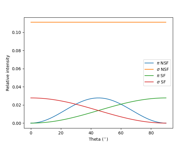
Plot
We now run through a few configurations specified in terms of incoming polarization angle \(\alpha\) (defined in radians w.r.t. the scattering plane), \(F\), plotting label, and plotting color.
fig, ax = plt.subplots()

config = [[0, F_NSF, r'$\pi$ NSF', 'C0'],
          [np.pi/2, F_NSF, r'$\sigma$ NSF', 'C1'],
          [0, F_SF, r'$\pi$ SF', 'C2'],
          [np.pi/2, F_SF, r'$\sigma$ SF', 'C3']]

for alpha, F, label, color in config:
    Is = np.array([get_I(thin, alpha, F) for thin in thins])
    ax.plot(thins, Is, label=label, color=color)

ax.legend()
ax.set_xlabel(r'Theta ($^\circ$)')
ax.set_ylabel('Relative intensity')
plt.show()
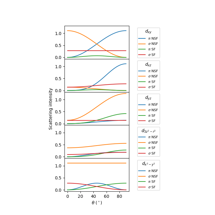
Run through orbitals
For completeness, let’s look at transitions from \(x^2-y^2\) to all other orbitals.
fig, axs = plt.subplots(5, 1, figsize=(7, 7),
                        sharex=True, sharey=True)

orbitals = ['$d_{3z^2-r^2}$', '$d_{xz}$', '$d_{yz}$',
            '$d_{x^2-y^2}$', '$d_{xy}$']
orbital_order = [4, 1, 2, 0, 3]

plot_index = 0
for ax, orbital_index in zip(axs, orbital_order):
    for spin_index, spin_label in zip([0, 1], ['NSF', 'SF']):
        excitedstate_vector = get_eigenvector(orbital_index, spin_index)
        F = get_F(groundstate_vector, excitedstate_vector)
        for alpha, pol_label in zip([0, np.pi/2], [r'$\pi$', r'$\sigma$']):
            Is = np.array([get_I(thin, alpha, F) for thin in thins])
            ax.plot(thins, Is*10, label=f'{pol_label} {spin_label}',
                    color=f'C{plot_index%4}')
            plot_index += 1
    ax.legend(title=orbitals[orbital_index], bbox_to_anchor=(1.1, 1),
              loc="upper left", fontsize=8)


axs[-1].set_xlabel(r'$\theta$ ($^\circ$)')
axs[2].set_ylabel('Scattering intensity')

fig.subplots_adjust(hspace=0, left=.3, right=.6)
plt.show()
Footnotes
Total running time of the script: (0 minutes 0.559 seconds)