Use scans with adaptive step sizes
Problem
Concentrate measurement in regions of high variability, taking larger strides through flat regions.
Approach
The plans in bluesky can be fully adaptive, determining one step at a time. A couple built-in plans provide this capability out of the box.
Example Solution
The adaptive_scan aims to maintain a certain delta in y between successive
steps through x. After each step, it accounts for the local derivative and
adjusts it step size accordingly. If it misses by a large margin, it takes a
step backward (if allowed).
See its documentation for a full list of paramters and their meanings. Here is working example:
We’ll add a LiveTable and a LivePlot.
In [1]: from bluesky.plans import adaptive_scan

In [2]: ad_scan = adaptive_scan([det], 'det', motor, -15, 10, .01, 5, .05, True)

In [3]: RE(ad_scan, [LiveTable(['det', 'motor']), LivePlot('det', 'motor', markersize=10, marker='o')])
+-----------+------------+------------+------------+
|   seq_num |       time |        det |      motor |
+-----------+------------+------------+------------+
|         1 | 17:01:12.4 |       0.00 |     -15.00 |
|         2 | 17:01:12.5 |       0.00 |     -12.50 |
|         3 | 17:01:12.5 |       0.00 |      -9.51 |
|         4 | 17:01:12.6 |       0.00 |      -6.11 |
|         5 | 17:01:12.6 |       0.06 |      -2.39 |
|         6 | 17:01:12.7 |       0.47 |       1.23 |
|         7 | 17:01:12.7 |       0.15 |      -1.95 |
|         8 | 17:01:12.7 |       0.10 |      -2.15 |
|         9 | 17:01:12.7 |       0.16 |      -1.90 |
|        10 | 17:01:12.8 |       0.15 |      -1.96 |
|        11 | 17:01:12.8 |       0.21 |      -1.77 |
|        12 | 17:01:12.8 |       0.19 |      -1.81 |
|        13 | 17:01:12.9 |       0.25 |      -1.66 |
|        14 | 17:01:12.9 |       0.32 |      -1.51 |
|        15 | 17:01:12.9 |       0.30 |      -1.55 |
|        16 | 17:01:13.0 |       0.36 |      -1.43 |
|        17 | 17:01:13.0 |       0.42 |      -1.33 |
|        18 | 17:01:13.0 |       0.48 |      -1.22 |
|        19 | 17:01:13.1 |       0.54 |      -1.12 |
|        20 | 17:01:13.1 |       0.60 |      -1.02 |
|        21 | 17:01:13.1 |       0.65 |      -0.92 |
|        22 | 17:01:13.2 |       0.71 |      -0.83 |
|        23 | 17:01:13.3 |       0.76 |      -0.74 |
|        24 | 17:01:13.3 |       0.81 |      -0.65 |
|        25 | 17:01:13.3 |       0.86 |      -0.56 |
|        26 | 17:01:13.4 |       0.90 |      -0.46 |
|        27 | 17:01:13.4 |       0.93 |      -0.37 |
|        28 | 17:01:13.4 |       0.97 |      -0.26 |
|        29 | 17:01:13.5 |       0.99 |      -0.15 |
|        30 | 17:01:13.5 |       1.00 |      -0.01 |
|        31 | 17:01:13.5 |       0.97 |       0.24 |
|        32 | 17:01:13.6 |       0.87 |       0.52 |
|        33 | 17:01:13.6 |       0.93 |       0.38 |
|        34 | 17:01:13.6 |       0.87 |       0.53 |
|        35 | 17:01:13.7 |       0.80 |       0.67 |
|        36 | 17:01:13.7 |       0.82 |       0.63 |
|        37 | 17:01:13.7 |       0.77 |       0.73 |
|        38 | 17:01:13.7 |       0.71 |       0.83 |
|        39 | 17:01:13.8 |       0.65 |       0.92 |
|        40 | 17:01:13.8 |       0.60 |       1.02 |
|        41 | 17:01:13.9 |       0.54 |       1.11 |
|        42 | 17:01:13.9 |       0.49 |       1.20 |
|        43 | 17:01:13.9 |       0.44 |       1.29 |
|        44 | 17:01:13.9 |       0.39 |       1.38 |
|        45 | 17:01:14.0 |       0.34 |       1.47 |
|        46 | 17:01:14.0 |       0.30 |       1.56 |
|        47 | 17:01:14.0 |       0.26 |       1.65 |
|        48 | 17:01:14.1 |       0.22 |       1.75 |
|        49 | 17:01:14.1 |       0.18 |       1.85 |
+-----------+------------+------------+------------+
|   seq_num |       time |        det |      motor |
+-----------+------------+------------+------------+
|        50 | 17:01:14.1 |       0.15 |       1.96 |
|        51 | 17:01:14.1 |       0.11 |       2.08 |
|        52 | 17:01:14.2 |       0.09 |       2.21 |
|        53 | 17:01:14.2 |       0.06 |       2.37 |
|        54 | 17:01:14.2 |       0.04 |       2.55 |
|        55 | 17:01:14.3 |       0.02 |       2.78 |
|        56 | 17:01:14.3 |       0.01 |       3.10 |
|        57 | 17:01:14.3 |       0.00 |       3.60 |
|        58 | 17:01:14.4 |       0.00 |       4.75 |
|        59 | 17:01:14.4 |       0.00 |       6.67 |
|        60 | 17:01:14.4 |       0.00 |       9.20 |
+-----------+------------+------------+------------+
generator adaptive_scan ['e93d28'] (scan num: 1)
Out[3]: ['e93d28bf-aff1-4c90-815c-c37a497acab8']
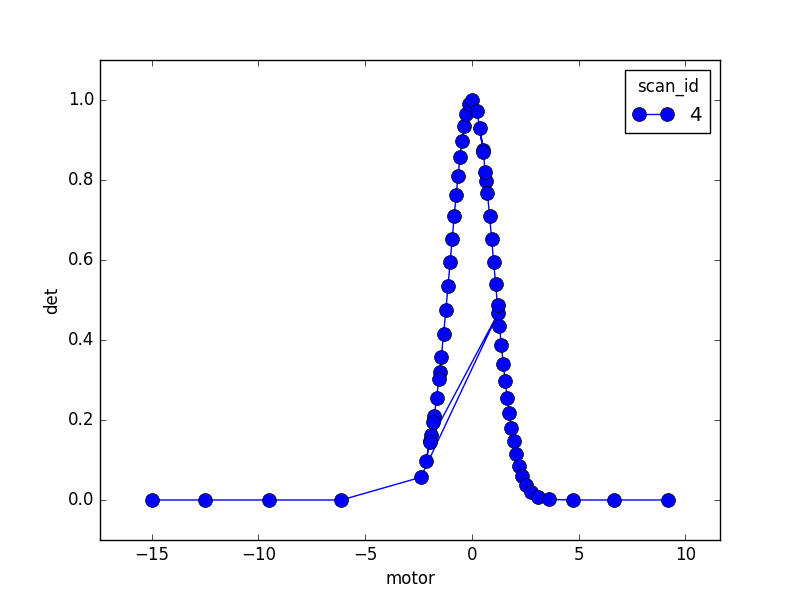
Observe how the scan lengthens its stride through the flat regions, oversteps through the peak, moves back, samples it with smaller steps, and gradually adopts a larger stride as the peak flattens out again.