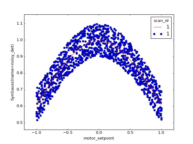
Re-scan until fit achieves desired confidence

Problem

Scan a peak and, in real time, fit Gaussian model to the data. Repeatedly re-scan the same region until the uncertainty in the Gaussian width parameter, sigma, is below some threshold.

Approach

Use callbacks.LiveFit() and callbacks.LiveFitPlot() to perform and visualize a non-linear least-squared fit.

Normally we would use plans.scan() to perform the 1D scan. In this case, we need something more sophisticated to incorporate adaptive logic that continues the scan until the fit attains sufficient confidence in sigma. We write our scan logic using the lower-level plans plans.abs_set() and plans.trigger_and_read().

Example Solution

import matplotlib.pyplot as plt
import numpy as np
import lmfit
from bluesky.plans import (subs_decorator, abs_set, trigger_and_read,
                           run_decorator, stage_decorator)
from bluesky.callbacks import LiveFit, LiveFitPlot, LivePlot
from bluesky.examples import motor, noisy_det


def errorbar(lmfit_result, param_name):
    # width of 95% conf interfal:
    ci = lmfit_result.conf_interval()
    return ci[param_name][-2][1] - ci[param_name][1][1]


def gaussian(x, A, sigma, x0):
    return A * np.exp(-(x - x0)**2 / (2 * sigma**2))


model = lmfit.Model(gaussian)
guess = {'A': 10,
         'x0': 1,
         'sigma': lmfit.Parameter('sigma', 3, min=0)}


def scan_gaussian(detectors, motor, start, stop, num):
    global lf
    main_detector = detectors[0]
    main_motor_field, *_ = motor.describe()
    lf = LiveFit(model, main_detector.name, {'x': main_motor_field}, guess)
    lfp = LiveFitPlot(lf, color='r', ax=plt.gca())
    lp = LivePlot(main_detector, main_motor_field,
                  linestyle='none', marker='o', ax=plt.gca())

    @subs_decorator([lfp, lp])
    @stage_decorator(list(detectors) + [motor])
    @run_decorator()
    def plan():
        while True:
            for step in np.linspace(start, stop, num):
                yield from abs_set(motor, step, wait=True)
                yield from trigger_and_read(list(detectors) + [motor])
            err = errorbar(lf.result, 'sigma')
            if err < .03:
                break

    yield from plan()


# Example usage:

RE(scan_gaussian([noisy_det], motor, -1, 1, 200))