Quickstart tutorial
If you are already familiar with multiplet calculations this page and our examples page are a good part to start. Otherwise, checkout our Pedagogical examples to learn the concepts behind how edrixs works. The first example explains Exact diagonalization.
Use edrixs as an ED calculator
edrixs can be used as a simple ED calculator to get eigenvalues (eigenvectors) of a many-body Hamiltonian with small size dimension (\(< 1,000\)). We will give an example to get eigenvalues for a \(t_{2g}\)-orbital system (\(l_{eff}=1\)). There are 6 orbitals including spin.
Launch your favorite python terminal:
>>> import edrixs
>>> import scipy
>>> norb = 6
>>> noccu = 2
>>> Ud, JH = edrixs.UJ_to_UdJH(4, 1)
>>> F0, F2, F4 = edrixs.UdJH_to_F0F2F4(Ud, JH)
>>> umat = edrixs.get_umat_slater('t2g', F0, F2, F4)
>>> emat = edrixs.atom_hsoc('t2g', 0.2)
>>> basis = edrixs.get_fock_bin_by_N(norb, noccu)
>>> H = edrixs.build_opers(4, umat, basis)
>>> e1, v1 = scipy.linalg.eigh(H)
>>> H += edrixs.build_opers(2, emat, basis)
>>> e2, v2 = scipy.linalg.eigh(H)
>>> print(e1)
[1. 1. 1. 1. 1. 1. 1. 1. 1. 3. 3. 3. 3. 3. 6.]
>>> print(e2)
[0.890519 0.890519 0.890519 0.890519 0.890519 1.1      1.1      1.1
 1.183391 3.009481 3.009481 3.009481 3.009481 3.009481 6.016609]
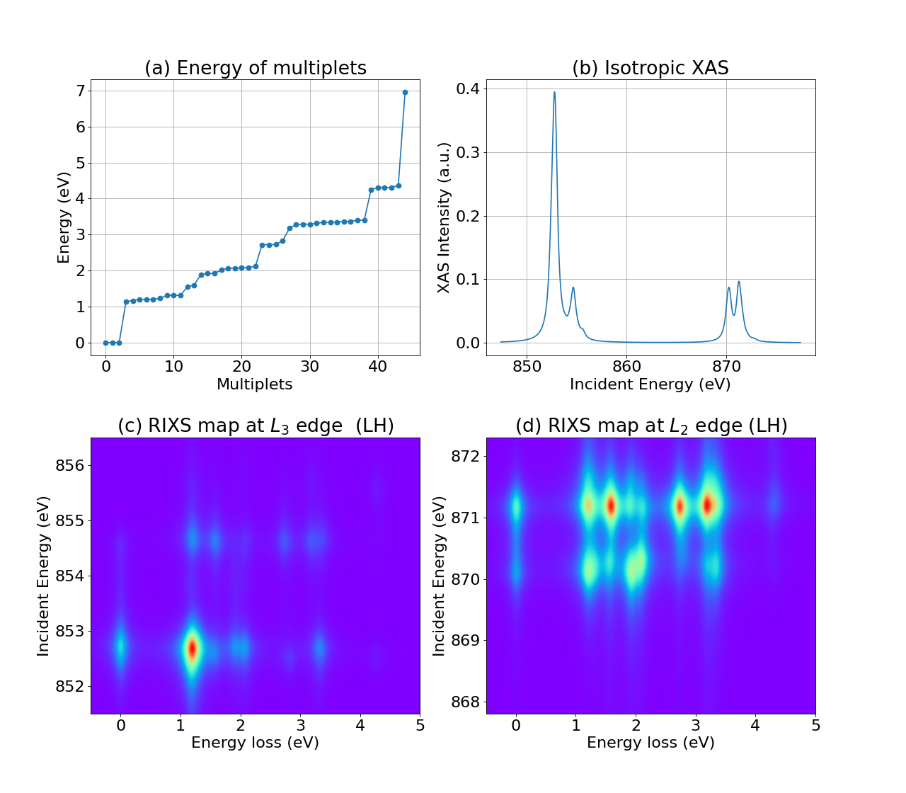
Hello RIXS!
This is a “Hello World!” example for RIXS simulations at Ni (\(3d^8\)) \(L_{2/3}\) edges. \(L_3\) means transition from Ni-\(2p_{3/2}\) to Ni-\(3d\), and \(L_2\) means transition from Ni-\(2p_{1/2}\) to Ni-\(3d\).
#!/usr/bin/env python

import numpy as np
import matplotlib.pyplot as plt
import matplotlib as mpl
import edrixs

# Setup parameters
# ----------------
# Number of occupancy of 3d shell
noccu = 8

res = edrixs.get_atom_data('Ni', v_name='3d', v_noccu=noccu, edge='L23')
name_i, slat_i = [list(i) for i in zip(*res['slater_i'])]
name_n, slat_n = [list(i) for i in zip(*res['slater_n'])]

# Slater integrals for initial Hamiltonian without core-hole
si = edrixs.rescale(slat_i, ([1, 2], [0.65]*2))
si[0] = edrixs.get_F0('d', si[1], si[2])    # F0_dd

# Slater integrals for intermediate Hamiltonian with core-hole
sn = edrixs.rescale(slat_n, ([1, 2, 4, 5, 6], [0.65, 0.65, 0.95, 0.7, 0.7]))
sn[0] = edrixs.get_F0('d', sn[1], sn[2])     # F0_dd
sn[3] = edrixs.get_F0('dp', sn[5], sn[6])    # F0_dp

slater = (si, sn)

# Spin-orbit coupling strengths
zeta_d_i = res['v_soc_i'][0]  # valence 3d electron without core-hole
zeta_d_n = res['v_soc_n'][0]  # valence 3d electron with core-hole
# E_{L2} - E_{L3} = 1.5 * zeta_p
zeta_p_n = (res['edge_ene'][0] - res['edge_ene'][1]) / 1.5  # core 2p electron

# Tetragonal crystal field
cf = edrixs.cf_tetragonal_d(ten_dq=1.3, d1=0.05, d3=0.2)

# Level shift of the core shell
off = 857.4

# Life time broadening
gamma_c = res['gamma_c'][1]  # core hole
gamma_f = 0.1  # final states

# Incident, scattered, azimuthal angles
# See Figure 1 of Y. Wang et al.,
# `Computer Physics Communications 243, 151-165 (2019)
# <https://doi.org/10.1016/j.cpc.2019.04.018>`_
# for the defintion of the scattering angles.
thin, thout, phi = 15 / 180.0 * np.pi, 75 / 180.0 * np.pi, 0.0

# Polarization types
poltype_xas = [('isotropic', 0.0)]  # for XAS
poltype_rixs = [('linear', 0, 'linear', 0), ('linear', 0, 'linear', np.pi/2.0)]  # for RIXS

# Energy grid
ominc_xas = np.linspace(off - 10, off + 20, 1000)  # for XAS
ominc_rixs_L3 = np.linspace(-5.9 + off, -0.9 + off, 100)  # incident energy at L3 edge
ominc_rixs_L2 = np.linspace(10.4 + off, 14.9 + off, 100)  # incident energy at L3 edge
eloss = np.linspace(-0.5, 5.0, 1000)  # energy loss for RIXS

# Run ED
eval_i, eval_n, trans_op = edrixs.ed_1v1c_py(
    ('d', 'p'), shell_level=(0.0, -off), v_soc=(zeta_d_i, zeta_d_n),
    c_soc=zeta_p_n, v_noccu=noccu, slater=slater, v_cfmat=cf
)

# Run XAS
xas = edrixs.xas_1v1c_py(
    eval_i, eval_n, trans_op, ominc_xas, gamma_c=gamma_c, thin=thin, phi=phi,
    pol_type=poltype_xas, gs_list=[0, 1, 2], temperature=300
)

# Run RIXS at L3 edge
rixs_L3 = edrixs.rixs_1v1c_py(
    eval_i, eval_n, trans_op, ominc_rixs_L3, eloss, gamma_c=gamma_c, gamma_f=gamma_f,
    thin=thin, thout=thout, phi=phi, pol_type=poltype_rixs, gs_list=[0, 1, 2],
    temperature=300
)

# Run RIXS at L2 edge
rixs_L2 = edrixs.rixs_1v1c_py(
    eval_i, eval_n, trans_op, ominc_rixs_L2, eloss, gamma_c=gamma_c, gamma_f=gamma_f,
    thin=thin, thout=thout, phi=phi, pol_type=poltype_rixs, gs_list=[0, 1, 2],
    temperature=300
)

# Plot
fig = plt.figure(figsize=(16, 14))
mpl.rcParams['font.size'] = 20

ax1 = plt.subplot(2, 2, 1)
plt.grid()
plt.plot(range(len(eval_i)), eval_i - min(eval_i), '-o')
plt.xlabel(r'Multiplets')
plt.ylabel(r'Energy (eV)')
plt.title(r'(a) Energy of multiplets')

ax2 = plt.subplot(2, 2, 2)
plt.grid()
plt.plot(ominc_xas, xas[:, 0], '-')
plt.xlabel(r'Incident Energy (eV)')
plt.ylabel(r'XAS Intensity (a.u.)')
plt.title(r'(b) Isotropic XAS')

ax3 = plt.subplot(2, 2, 3)
plt.imshow(np.sum(rixs_L3, axis=2),
           extent=[min(eloss), max(eloss), min(ominc_rixs_L3), max(ominc_rixs_L3)],
           origin='lower', aspect='auto', cmap='rainbow', interpolation='gaussian')
plt.xlabel(r'Energy loss (eV)')
plt.ylabel(r'Incident Energy (eV)')
plt.title(r'(c) RIXS map at $L_3$ edge  (LH)')

ax4 = plt.subplot(2, 2, 4)
plt.imshow(np.sum(rixs_L2, axis=2),
           extent=[min(eloss), max(eloss), min(ominc_rixs_L2), max(ominc_rixs_L2)],
           origin='lower', aspect='auto', cmap='rainbow', interpolation='gaussian')
plt.xlabel(r'Energy loss (eV)')
plt.ylabel(r'Incident Energy (eV)')
plt.title(r'(d) RIXS map at $L_2$ edge (LH)')

plt.subplots_adjust(left=0.1, right=0.9, bottom=0.1, top=0.9, wspace=0.2, hspace=0.3)
plt.show()