Use scans with adaptive step sizes

Problem

Concentrate measurement in regions of high variability, taking larger strides through flat regions.

Approach

The plans in bluesky can be fully adaptive, determining one step at a time. A couple built-in plans provide this capability out of the box.

Example Solution

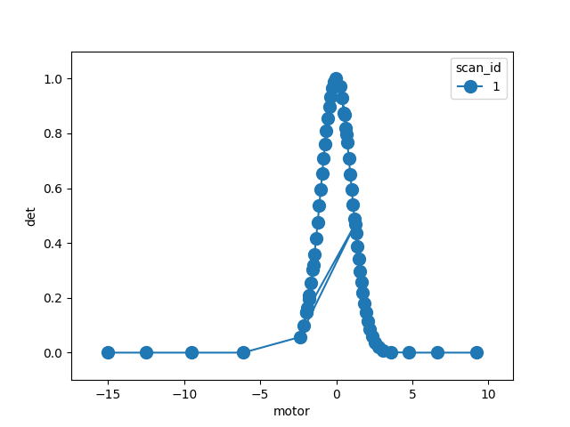
The bluesky.plans.adaptive_scan() aims to maintain a certain delta in y between successive steps through x. After each step, it accounts for the local derivative and adjusts it step size accordingly. If it misses by a large margin, it takes a step backward (if allowed).

import matplotlib.pyplot as plt

from bluesky import RunEngine
from bluesky.plans import adaptive_scan
from bluesky.callbacks import LivePlot
from ophyd.sim import motor, det

# Do this if running the example interactively;
# skip it when building the documentation.
import os
if 'BUILDING_DOCS' not in os.environ:
    from bluesky.utils import install_qt_kicker  # for notebooks, qt -> nb
    install_qt_kicker()
    plt.ion()
    det.exposure_time = 0.5  # simulate slow exposures

RE = RunEngine({})

RE(adaptive_scan([det], 'det', motor,
                 start=-15,
                 stop=10,
                 min_step=0.01,
                 max_step=5,
                 target_delta=.05,
                 backstep=True),
   LivePlot('det', 'motor', markersize=10, marker='o'))

Observe how the scan lengthens its stride through the flat regions, oversteps through the peak, moves back, samples it with smaller steps, and gradually adopts a larger stride as the peak flattens out again.