Live Visualization and Processing

Overview of Callbacks

As the RunEngine executes a plan, it organizes metadata and data into Documents, Python dictionaries organized in a specified but flexible way. Each time a new Document is created, the RunEngine passes it to a list of functions. These functions can do anything: store the data to disk, print a line of text to the screen, add a point to a plot, or even transfer the data to a cluster for immediate processing. These functions are called “callbacks.”

We “subscribe” callbacks to the live stream of Documents coming from the RunEngine. You can think of a callback as a self-addressed stamped envelope: it tells the RunEngine, “When you create a Document, send it to this function for processing.”

Callback functions are run in a blocking fashion: data acquisition cannot continue until they return. For light tasks like simple plotting or critical tasks like sending the data to a long-term storage medium, this behavior is desirable. It is easy to debug and it guarantees that critical errors will be noticed immediately. But heavy computational tasks — anything that takes more than about 0.2 seconds to finish — should be executed in a separate process or server so that they do not hold up data acquisition. Bluesky provides nice tooling for this use case — see Subscriptions in Separate Processes or Host with 0MQ.

Simplest Working Example

This example passes every Document to the print function, printing each Document as it is generated during data collection.

from bluesky.plans import count
from ophyd.sim import det

RE(count([det]), print)

The print function is a blunt instrument; it dumps too much information to the screen. See LiveTable below for a more refined option.

Ways to Invoke Callbacks

Interactively

As in the simple example above, pass a second argument to the RunEngine. For some callback function cb, the usage is:

RE(plan(), cb))

A working example:

from ophyd.sim import det, motor
from bluesky.plans import scan
from bluesky.callbacks import LiveTable
dets = [det]
RE(scan(dets, motor, 1, 5, 5), LiveTable(dets))

A list of callbacks — [cb1, cb2] — is also accepted; see Filtering by Document Type, below, for additional options.

Persistently

The RunEngine keeps a list of callbacks to apply to every plan it executes. For example, the callback that saves the data to a database is typically invoked this way. For some callback function cb, the usage is:

RE.subscribe(cb)

This step is usually performed in a startup file (i.e., IPython profile).

RunEngine.subscribe(func, name='all')

Register a callback function to consume documents.

Changed in version 0.10.0: The order of the arguments was swapped and the name argument has been given a default value, 'all'. Because the meaning of the arguments is unambiguous (they must be a callable and a string, respectively) the old order will be supported indefinitely, with a warning.

Parameters

func: callable

expecting signature like f(name, document) where name is a string and document is a dict

name{‘all’, ‘start’, ‘descriptor’, ‘event’, ‘stop’}, optional

the type of document this function should receive (‘all’ by default)

Returns

tokenint

an integer ID that can be used to unsubscribe

See also

RunEngine.unsubscribe()

RunEngine.unsubscribe(token)

Unregister a callback function its integer ID.

Parameters

tokenint

the integer ID issued by RunEngine.subscribe()

See also

RunEngine.subscribe()

Through a plan

Use the subs_decorator plan preprocessor to attach callbacks to a plan so that they are subscribed every time it is run.

In this example, we define a new plan, plan2, that adds some callback cb to some existing plan, plan1.

from bluesky.preprocessors import subs_decorator

@subs_decorator(cb)
def plan2():
    yield from plan1()

or, equivalently,

plan2 = subs_decorator(cb)(plan1)

For example, to define a variant of scan that includes a table by default:

from bluesky.plans import scan
from bluesky.preprocessors import subs_decorator

def my_scan(detectors, motor, start, stop, num, *, per_step=None, md=None):
    "This plan takes the same arguments as `scan`."

    table = LiveTable([motor] + list(detectors))

    @subs_decorator(table)
    def inner():
        yield from scan(detectors, motor, start, stop, num,
                        per_step=per_step, md=md)

    yield from inner()

Callbacks for Visualization & Fitting

LiveTable

As each data point is collected (i.e., as each Event Document is generated) a row is added to the table. Demo:

In [1]: from bluesky.plans import scan

In [2]: from ophyd.sim import motor, det

In [3]: from bluesky.callbacks import LiveTable

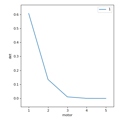
In [4]: RE(scan([det], motor, 1, 5, 5), LiveTable([motor, det]))


+-----------+------------+------------+----------------+------------+
|   seq_num |       time |      motor | motor_setpoint |        det |
+-----------+------------+------------+----------------+------------+
|         1 | 03:13:46.3 |      1.000 |          1.000 |      0.607 |
|         2 | 03:13:46.3 |      2.000 |          2.000 |      0.135 |
|         3 | 03:13:46.3 |      3.000 |          3.000 |      0.011 |
|         4 | 03:13:46.3 |      4.000 |          4.000 |      0.000 |
|         5 | 03:13:46.4 |      5.000 |          5.000 |      0.000 |
+-----------+------------+------------+----------------+------------+
generator scan ['2e1548c2'] (scan num: 1)


Out[4]: ('2e1548c2-3e2d-4766-a7d7-0f7ece791bbb',)

Pass an empty list of columns to show simply ‘time’ and ‘seq_num’ (sequence number).

LiveTable([])

In the demo above, we passed in a list of device(s), like so:

LiveTable([motor])

Internally, LiveTable obtains the name(s) of the field(s) produced by reading motor. You can do this yourself too:

In [5]: list(motor.describe().keys())
Out[5]: ['motor', 'motor_setpoint']

In the general case, a device can produce tens or even hundreds of separate readings, and it can be useful to spell out specific fields rather than a whole device.

# the field 'motor', in quotes, not the device, motor
LiveTable(['motor'])

In fact, almost all other callbacks (including LivePlot (for scalar data)) require a specific field. They will not accept a device because it may have more than one field.

class bluesky.callbacks.LiveTable(fields, *, stream_name='primary', print_header_interval=50, min_width=12, default_prec=3, extra_pad=1, separator_lines=True, logbook=None, out=<built-in function print>)

Live updating table

Parameters

fieldslist

List of fields to add to the table.

stream_namestr, optional

The event stream to watch for

print_header_intervalint, optional

Reprint the header every this many lines, defaults to 50

min_widthint, optional

The minimum width is spaces of the data columns. Defaults to 12

default_precint, optional

Precision to use if it can not be found in descriptor, defaults to 3

extra_padint, optional

Number of extra spaces to put around the printed data, defaults to 1

separator_linesbool, optional

Add empty lines before and after the printed table, default True

logbookcallable, optional

Must take a sting as the first positional argument

def logbook(input_str):

pass

outcallable, optional

Function to call to ‘print’ a line. Defaults to print

Aside: Making plots update live

Note

If you are a user working with a pre-configured setup, you can probably skip this. Come back if your plots are not appearing / updating.

This configuration is typically performed in an IPython profile startup script so that is happens automatically at startup time.

To make plots live-update while the RunEngine is executing a plan, you have run this command once. In an IPython terminal, the command is:

%matplotlib qt
from bluesky.utils import install_qt_kicker
install_qt_kicker()

If you are using a Jupyter notebook, the command is:

%matplotlib notebook
from bluesky.utils import install_nb_kicker
install_nb_kicker()

Why? The RunEngine and matplotlib (technically, matplotlib’s Qt backend) both use an event loop. The RunEngine takes control of the event loop while it is executing a plan. The kicker function periodically “kicks” the Qt event loop so that the plots can re-draw while the RunEngine is running.

The %matplotlib ... command is standard setup, having nothing to do with bluesky in particular. See the relevant section of the IPython documentation for details.

bluesky.utils.install_kicker(loop=None, update_rate=0.03)

Install a periodic callback to integrate drawing and asyncio event loops.

This dispatches to install_qt_kicker() or install_nb_kicker() depending on the current matplotlib backend.

Parameters

loopevent loop, optional

update_ratenumber

Seconds between periodic updates. Default is 0.03.

bluesky.utils.install_qt_kicker(loop=None, update_rate=0.03)

Install a periodic callback to integrate Qt and asyncio event loops.

DEPRECATED: This functionality is now handled automatically by default and is configurable via the RunEngine’s new during_task parameter. Calling this function now has no effect. It will be removed in a future release of bluesky.

Parameters

loopevent loop, optional

update_ratenumber

Seconds between periodic updates. Default is 0.03.

bluesky.utils.install_nb_kicker(loop=None, update_rate=0.03)

Install a periodic callback to integrate ipykernel and asyncio event loops.

It is safe to call this function multiple times.

Parameters

loopevent loop, optional

update_ratenumber

Seconds between periodic updates. Default is 0.03.

LivePlot (for scalar data)

Plot scalars. Example:

from bluesky.plans import scan
from ophyd.sim import det, motor
from bluesky.callbacks.mpl_plotting import LivePlot

RE(scan([det], motor, -5, 5, 30), LivePlot('det', 'motor'))

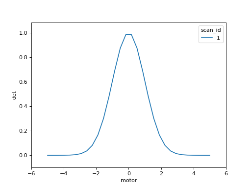
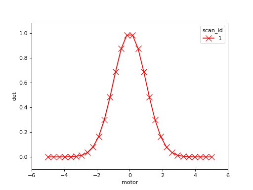
To customize style, pass in any matplotlib line style keyword argument. (LivePlot will pass it through to Axes.plot.) Example:

RE(scan([det], motor, -5, 5, 30),
   LivePlot('det', 'motor', marker='x', markersize=10, color='red'))

class bluesky.callbacks.mpl_plotting.LivePlot(y, x=None, *, legend_keys=None, xlim=None, ylim=None, ax=None, fig=None, epoch='run', **kwargs)

Build a function that updates a plot from a stream of Events.

Note: If your figure blocks the main thread when you are trying to scan with this callback, call plt.ion() in your IPython session.

Parameters

ystr

the name of a data field in an Event

xstr, optional

the name of a data field in an Event, or ‘seq_num’ or ‘time’ If None, use the Event’s sequence number. Special case: If the Event’s data includes a key named ‘seq_num’ or ‘time’, that takes precedence over the standard ‘seq_num’ and ‘time’ recorded in every Event.

legend_keyslist, optional

The list of keys to extract from the RunStart document and format in the legend of the plot. The legend will always show the scan_id followed by a colon (“1: “). Each

xlimtuple, optional

passed to Axes.set_xlim

ylimtuple, optional

passed to Axes.set_ylim

axAxes, optional

matplotib Axes; if none specified, new figure and axes are made.

figFigure, optional

deprecated: use ax instead

epoch{‘run’, ‘unix’}, optional

If ‘run’ t=0 is the time recorded in the RunStart document. If ‘unix’, t=0 is 1 Jan 1970 (“the UNIX epoch”). Default is ‘run’.

All additional keyword arguments are passed through to ``Axes.plot``.

Examples

>>> my_plotter = LivePlot('det', 'motor', legend_keys=['sample'])
>>> RE(my_scan, my_plotter)

Live Image

class bluesky.callbacks.broker.LiveImage(field, *, db=None, cmap=None, norm=None, limit_func=None, auto_redraw=True, interpolation=None, window_title=None)

Stream 2D images in a cross-section viewer.

Parameters

fieldstring

name of data field in an Event

fs: Registry instance

The Registry instance to pull the data from

cmapstr, colormap, or None

color map to use. Defaults to gray

normNormalize or None

Normalization function to use

limit_funccallable, optional

function that takes in the image and returns clim values

auto_redrawbool, optional

interpolationstr, optional

Interpolation method to use. List of valid options can be found in CrossSection2DView.interpolation

LiveGrid (gridded heat map)

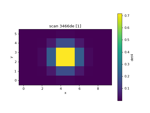
Plot a scalar value as a function of two variables on a regular grid. Example:

from bluesky.plans import grid_scan
from ophyd.sim import det4, motor1, motor2
from bluesky.callbacks.mpl_plotting import LiveGrid

RE(grid_scan([det4], motor1, -3, 3, 6, motor2, -5, 5, 10, False),
   LiveGrid((6, 10), 'det4'))

class bluesky.callbacks.mpl_plotting.LiveGrid(raster_shape, I, *, clim=None, cmap='viridis', xlabel='x', ylabel='y', extent=None, aspect='equal', ax=None, x_positive='right', y_positive='up', **kwargs)

Plot gridded 2D data in a “heat map”.

This assumes that readings are placed on a regular grid and can be placed into an image by sequence number. The seq_num is used to determine which pixel to fill in.

For non-gridded data with arbitrary placement, use bluesky.callbacks.mpl_plotting.LiveScatter().

This simply wraps around a AxesImage.

Parameters

raster_shapetuple

The (row, col) shape of the raster

Istr

The field to use for the color of the markers

climtuple, optional

The color limits

cmapstr or colormap, optional

The color map to use

xlabel, ylabelstr, optional

Labels for the x and y axis

extentscalars (left, right, bottom, top), optional

Passed through to matplotlib.axes.Axes.imshow()

aspectstr or float, optional

Passed through to matplotlib.axes.Axes.imshow()

axAxes, optional

matplotib Axes; if none specified, new figure and axes are made.

x_positive: string, optional

Defines the positive direction of the x axis, takes the values ‘right’ (default) or ‘left’.

y_positive: string, optional

Defines the positive direction of the y axis, takes the values ‘up’ (default) or ‘down’.

See also

bluesky.callbacks.mpl_plotting.LiveScatter

LiveScatter (scattered heat map)

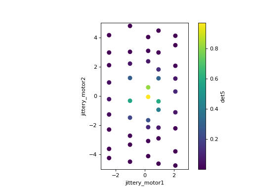
Plot a scalar value as a function of two variables. Unlike bluesky.callbacks.mpl_plotting.LiveGrid, this does not assume a regular grid. Example:

from bluesky.plans import grid_scan
from ophyd.sim import det5, jittery_motor1, jittery_motor2
from bluesky.callbacks.mpl_plotting import LiveScatter

# The 'jittery' example motors won't go exactly where they are told to go.

RE(grid_scan([det5],
                      jittery_motor1, -3, 3, 6,
                      jittery_motor2, -5, 5, 10, False),
   LiveScatter('jittery_motor1', 'jittery_motor2', 'det5',
            xlim=(-3, 3), ylim=(-5, 5)))

class bluesky.callbacks.mpl_plotting.LiveScatter(x, y, I, *, xlim=None, ylim=None, clim=None, cmap='viridis', ax=None, **kwargs)

Plot scattered 2D data in a “heat map”.

Alternatively, if the data is placed on a regular grid, you can use bluesky.callbacks.mpl_plotting.LiveGrid().

This simply wraps around a PathCollection as generated by scatter.

Parameters

x, ystr

The fields to use for the x and y data

Istr

The field to use for the color of the markers

xlim, ylim, climtuple, optional

The x, y and color limits respectively

cmapstr or colormap, optional

The color map to use

axAxes, optional

matplotib Axes; if none specified, new figure and axes are made.

All additional keyword arguments are passed through to ``Axes.scatter``.

See also

bluesky.callbacks.mpl_plotting.LiveGrid

LiveFit

Perform a nonlinear least squared best fit to the data with a user-defined model function. The function can depend on any number of independent variables. We integrate with the package lmfit, which provides a nice interface for NLS minimization.

In this example, we fit a Gaussian to detector readings as a function of motor position. First, define a Gaussian function, create an lmfit.Model from it, and provide initial guesses for the parameters.

import numpy as np
import lmfit

def gaussian(x, A, sigma, x0):
    return A*np.exp(-(x - x0)**2/(2 * sigma**2))

model = lmfit.Model(gaussian)
init_guess = {'A': 2,
              'sigma': lmfit.Parameter('sigma', 3, min=0),
              'x0': -0.2}

The guesses can be given as plain numbers or as lmfit.Parameter objects, as in the case of ‘sigma’ above, to specify constraints.

To integrate with the bluesky we need to provide:

• the field with the dependent variable (in this example, 'noisy_det')

• a mapping between the name(s) of independent variable(s) in the function ('x') to the corresponding field(s) in the data ('motor')

• any initial guesses expected by the model (defined above)

from bluesky.plans import scan
from ophyd.sim import motor, noisy_det
from bluesky.callbacks import LiveFit

lf = LiveFit(model, 'noisy_det', {'x': 'motor'}, init_guess)

RE(scan([noisy_det], motor, -1, 1, 100), lf)
# best-fit values for 'A', 'sigma' and 'x0' are in lf.result.values

The fit results are accessible in the result attribute of the callback. For example, the center of the Gaussian is lf.result.values['x0']. This could be used in a next step, like so:

x0 = lf.result.values['x0']
RE(scan([noisy_det], x0 - 1, x0 + 1, 100))

Refer the lmfit documentation for more about result.

This example uses a model with two independent variables, x and y.

from ophyd.sim import motor1, motor2, det4

def gaussian(x, y, A, sigma, x0, y0):
    return A*np.exp(-((x - x0)**2 + (y - y0)**2)/(2 * sigma**2))

# Specify the names of the independent variables to Model.
model = lmfit.Model(gaussian, ['x', 'y'])

init_guess = {'A': 2,
              'sigma': lmfit.Parameter('sigma', 3, min=0),
              'x0': -0.2,
              'y0': 0.3}

lf = LiveFit(model, 'det4', {'x': 'motor1', 'y': 'motor2'}, init_guess)

# Scan a 2D mesh.
RE(grid_scan([det4], motor1, -1, 1, 20, motor2, -1, 1, 20, False),
   lf)

By default, the fit is recomputed every time a new data point is available. See the API documentation below for other options. Fitting does not commence until the number of accumulated data points is equal to the number of free parameters in the model.

class bluesky.callbacks.LiveFit(model, y, independent_vars, init_guess=None, *, update_every=1)

Fit a model to data using nonlinear least-squares minimization.

Parameters

modellmfit.Model

ystring

name of the field in the Event document that is the dependent variable

independent_varsdict

map the independent variable name(s) in the model to the field(s) in the Event document; e.g., {'x': 'motor'}

init_guessdict, optional

initial guesses for other values, if expected by model; e.g., {'sigma': 1}

update_everyint or None, optional

How often to recompute the fit. If None, do not compute until the end. Default is 1 (recompute after each new point).

Attributes

resultlmfit.ModelResult

LiveFitPlot

This is a variation on LivePlot that plots the best fit curve from LiveFit. It applies to 1D model functions only.

Repeating the example from LiveFit above, adding a plot:

# same as above...

import numpy as np
import lmfit
from bluesky.plans import scan
from ophyd.sim import motor, noisy_det
from bluesky.callbacks import LiveFit

def gaussian(x, A, sigma, x0):
    return A*np.exp(-(x - x0)**2/(2 * sigma**2))

model = lmfit.Model(gaussian)
init_guess = {'A': 2,
              'sigma': lmfit.Parameter('sigma', 3, min=0),
              'x0': -0.2}

lf = LiveFit(model, 'noisy_det', {'x': 'motor'}, init_guess)

# now add the plot...

from bluesky.callbacks.mpl_plotting import LiveFitPlot
lpf = LiveFitPlot(lf, color='r')

RE(scan([noisy_det], motor, -1, 1, 100), lfp)

# Notice that we did'nt need to subscribe lf directly, just lfp.
# But, as before, the results are in lf.result.

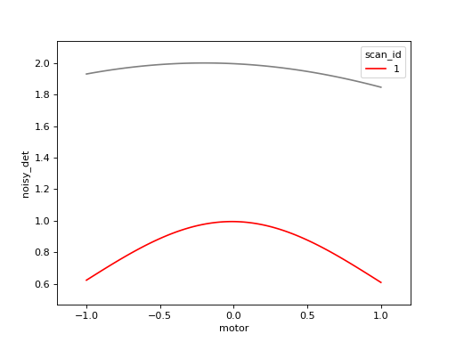
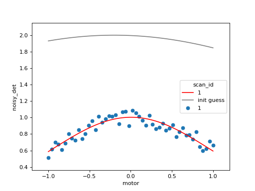
We can use the standard LivePlot to show the data on the same axes. Notice that they can styled independently.

import matplotlib.pyplot as plt

fig, ax = plt.subplots()  # explitly create figure, axes to use below
lfp = LiveFitPlot(lf, ax=ax, color='r')
lp = LivePlot('noisy_det', 'motor', ax=ax, marker='o', linestyle='none')

RE(scan([noisy_det], motor, -1, 1, 100), [lp, lfp])

class bluesky.callbacks.mpl_plotting.LiveFitPlot(livefit, *, num_points=100, legend_keys=None, xlim=None, ylim=None, ax=None, **kwargs)

Add a plot to an instance of LiveFit.

Note: If your figure blocks the main thread when you are trying to scan with this callback, call plt.ion() in your IPython session.

Parameters

livefitLiveFit

an instance of LiveFit

num_pointsint, optional

number of points to sample when evaluating the model; default 100

legend_keyslist, optional

The list of keys to extract from the RunStart document and format in the legend of the plot. The legend will always show the scan_id followed by a colon (“1: “). Each

xlimtuple, optional

passed to Axes.set_xlim

ylimtuple, optional

passed to Axes.set_ylim

axAxes, optional

matplotib Axes; if none specified, new figure and axes are made.

All additional keyword arguments are passed through to ``Axes.plot``.

PeakStats

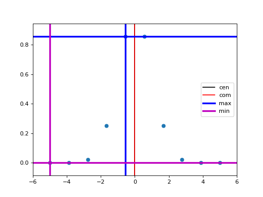
Compute statistics of peak-like data. Example:

from bluesky.callbacks.fitting import PeakStats
from ophyd.sim import motor, det
from bluesky.plans import scan

ps = PeakStats('motor', 'det')
RE(scan([det], motor, -5, 5, 10), ps)

Now attributes of ps, documented below, contain various peak statistics. There is also a convenience function for plotting:

from bluesky.callbacks.mpl_plotting import plot_peak_stats

plot_peak_stats(ps)

class bluesky.callbacks.fitting.PeakStats(x, y, edge_count=None)

Compute peak statsitics after a run finishes.

Results are stored in the attributes.

Parameters

xstring

field name for the x variable (e.g., a motor)

ystring

field name for the y variable (e.g., a detector)

edge_countint or None, optional

If not None, number of points at beginning and end to use for quick and dirty background subtraction.

Notes

It is assumed that the two fields, x and y, are recorded in the same Event stream.

Attributes

comcenter of mass

cenmid-point between half-max points on each side of the peak

maxx location of y maximum

minx location of y minimum

crossingscrosses between y and middle line, which is

((np.max(y) + np.min(y)) / 2). Users can estimate FWHM based on those info.

fwhmthe computed full width half maximum (fwhm) of a peak.

The distance between the first and last crossing is taken to be the fwhm.

bluesky.callbacks.mpl_plotting.plot_peak_stats(peak_stats, ax=None)

Plot data and various peak statistics.

Parameters

peak_statsPeakStats

axmatplotlib.Axes, optional

Returns

artsdict

dictionary of matplotlib Artist objects, for further styling

Best-Effort Callback

Warning

This is a new, experimental feature. It will likely be changed in future releases in a way that is not backward-compatible.

This is meant to be permanently subscribed to the RunEngine like so:

# one-time configuration
from bluesky.callbacks.best_effort import BestEffortCallback
bec = BestEffortCallback()
RE.subscribe(bec)

It provides best-effort plots and visualization for any plan. It uses the ‘hints’ key provided by the plan, if present. (See the source code of the plans in bluesky.plans for examples.)

In [6]: from ophyd.sim import det1, det2

In [7]: from bluesky.plans import scan

In [8]: dets = [det1, det2]

In [9]: RE(scan(dets, motor, 1, 5, 5))  # automatically prints table, shows plot


Transient Scan ID: 2     Time: 2020-12-15 03:14:10
Persistent Unique Scan ID: 'cc6fd923-11d6-4aef-8fc6-b7f8b114cfa2'
New stream: 'primary'
+-----------+------------+------------+------------+------------+
|   seq_num |       time |      motor |       det2 |       det1 |
+-----------+------------+------------+------------+------------+
|         1 | 03:14:11.1 |      1.000 |      0.271 |      0.000 |
|         2 | 03:14:11.2 |      2.000 |      0.271 |      0.000 |
|         3 | 03:14:11.3 |      3.000 |      0.271 |      0.000 |
|         4 | 03:14:11.4 |      4.000 |      0.271 |      0.000 |
|         5 | 03:14:11.5 |      5.000 |      0.271 |      0.000 |
+-----------+------------+------------+------------+------------+
generator scan ['cc6fd923'] (scan num: 2)



Out[9]: ('cc6fd923-11d6-4aef-8fc6-b7f8b114cfa2',)

Use these methods to toggle on or off parts of the functionality.

BestEffortCallback(*[, fig_factory, …])
BestEffortCallback.enable_heading()	Print timestamp and IDs at the top of a run.
BestEffortCallback.disable_heading()	Opposite of enable_heading()
BestEffortCallback.enable_table()	Print hinted readings from the ‘primary’ stream in a LiveTable.
BestEffortCallback.disable_table()	Opposite of enable_table()
BestEffortCallback.enable_baseline()	Print hinted fields from the ‘baseline’ stream.
BestEffortCallback.disable_baseline()	Opposite of enable_baseline()
BestEffortCallback.enable_plots()	Plot hinted fields from all streams not in noplot_streams.
BestEffortCallback.disable_plots()	Do not plot anything.

Blacklist plotting certain streams using the bec.noplot_streams attribute, which is a list of stream names. The blacklist is set to ['baseline'] by default.

The attribute bec.overplot can be used to control whether line plots for subsequent runs are plotted on the same axes. It is True by default. Overplotting only occurs if the names of the axes are the same from one plot to the next.

Peak Stats

For each plot, simple peak-fitting is performed in the background. Of course, it may or may not be applicable depending on your data, and it is not shown by default. To view fitting annotations in a plot, click the plot area and press Shift+P. (Lowercase p is a shortcut for “panning” the plot.)

To access the peak-fit statistics programmatically, use bec.peaks.

Hints

The best-effort callback aims to print and plot useful information without being overwhelmingly comprehensive. Its usefulness is improved and tuned by the hints attribute on devices (if available) and hints metadata injected by plans (if available). If either or both of these are not available, the best-effort callback still makes a best effort to display something useful.

The contents of hints do not at all affect what data is saved. The content only affect what is displayed automatically by the best-effort callback and other tools that opt to look at the hints. Additional callbacks may still be set up for live or post-facto visualization or processing that do more specific things without relying on hints.

The hints attribute or property on devices is a dictionary with the key 'fields' mapped to a list of fields.

On movable devices such as motors or temperature controllers, these fields are expected to comprise the independent axes of the device. A motor that reads the fields ['x', 'x_setpoint'] might provide the hint {'fields': ['x']} to indicate that it has one independent axis and that the field x is the best representation of its value.

A readable device might report many fields like ['chan1', 'chan2', 'chan3', 'chan4', 'chan5'] but perhaps only a couple are usually interesting. A useful hint might narrow them down to {'fields': ['chan1', 'chan2']} so that a “best-effort” plot does not display an overwhelming amount of information.

The hints provided by the devices are read by the RunEngine and collated in the Event Descriptor documents.

The plans generally know which devices are being used as dependent and independent variables (i.e., which are being “scanned” over), and they may provide this information via a 'hints' metadata key that they inject into the start document along with the rest of their metadata. Examples:

# The pattern is
# {'dimensions': [(fields, stream_name), (fields, stream_name), ...]}

# a scan over time
{'dimensions': [(('time',), 'primary')]}

# a one-dimensional scan
{'dimensions': [(motor.hints['fields'], 'primary')]}

# a two-dimensional scan
{'dimensions': [(x_motor.hints['fields'], 'primary'),
                (y_motor.hints['fields'], 'primary')]}

# an N-dimensional scan
{'dimensions': [(motor.hints['fields'], 'primary') for motor in motors]}

It’s possible to adjust hints interactively, but they are generally intended to be set in a startup file. Err on the side of displaying more information than you need to see, and you will rarely need to adjust them.

Plans may also hint that their data is sampled on a regular rectangular grid via the hint {'gridding': 'rectilinear'}. This is useful, for example, for decided whether to visualize 2D data with LiveGrid or with LiveScatter.

Callback for Export

Exporting Image Data as TIFF Files

First, compose a filename template. The template can include metadata or event data from the scan.

# a template that includes the scan ID and sequence number in each filename
template = "output_dir/{start[scan_id]}_{event[seq_num]}.tiff"

# a template that sorts files into directories based user and scan ID
template = "output_dir/{start[user]}/{start[scan_id]}/{event[seq_num]}.tiff"

# a more complex template includes actual measurements in the filenames
template = ("output_dir/{start[scan_id]}_{start[sample_name]}_"
            "{event[data][temperature]}_{event[seq_num]}.tiff")

Above, we are using a Python language feature called format strings. Notice that inside the curly brackets we don’t use quotes around the key names; it’s {event[seq_num]} not {event['seq_num']}.

If each image data point is actually a stack of 2D image planes, the template must also include {i}, which will count through the image planes in the stack.

Note

Most metadata comes from the “start” document, hence start.scan_id above. Review the Documents section for details.

Create a callback that exports TIFFs using your template.

from bluesky.callbacks.broker import LiveTiffExporter

exporter = LiveTiffExporter('image', template)

Finally, to export all the images from a run when it finishes running, wrap the exporter in post_run and subscribe.

from bluesky.callbacks.broker import post_run

RE.subscribe(post_run(exporter))

It also possible to write TIFFs live, hence the name LiveTiffExporter, but there is an important disadvantage to doing this subscription in the same process: progress of the experiment may be intermittently slowed while data is written to disk. In some circumstances, this affect on the timing of the experiment may not be acceptable.

RE.subscribe(exporter)

There are more configuration options available, as given in detail below. It is recommended to use these expensive callbacks in a separate process.

class bluesky.callbacks.broker.LiveTiffExporter(field, template, dryrun=False, overwrite=False, db=None)

Save TIFF files.

Incorporate metadata and data from individual data points in the filenames.

Parameters

fieldstr

a data key, e.g., ‘image’

templatestr

A templated file path, where curly brackets will be filled in with the attributes of ‘start’, ‘event’, and (for image stacks) ‘i’, a sequential number. e.g., “dir/scan{start[scan_id]}_by_{start[experimenter]}_{i}.tiff”

dryrunbool

default to False; if True, do not write any files

overwritebool

default to False, raising an OSError if file exists

dbBroker, optional

The databroker instance to use, if not provided use databroker singleton

Attributes

filenameslist of filenames written in ongoing or most recent run

Export All Data and Metadata in an HDF5 File

A Stop Document is emitted at the end of every run. Subscribe to it, using it as a cue to load the dataset via the DataBroker and export an HDF5 file using suitcase.

Working example:

from databroker import DataBroker as db
import suitcase

def suitcase_as_callback(name, doc):
    if name != 'stop':
        return
    run_start_uid = doc['run_start']
    header = db[run_start_uid]
    filename = '{}.h5'.format(run_start_uid)
    suitcase.export(header, filename)

RE.subscribe(suitcase_as_callback, 'stop')

Export Metadata to the Olog

The Olog (“operational log”) is an electronic logbook. We can use a callback to automatically generate log entries at the beginning of a run. The Python interface to Olog is not straightforward, so there is some boilerplate:

from functools import partial
from pyOlog import SimpleOlogClient
from bluesky.callbacks.olog import logbook_cb_factory

# Set up the logbook. This configures bluesky's summaries of
# data acquisition (scan type, ID, etc.).

LOGBOOKS = ['Data Acquisition']  # list of logbook names to publish to
simple_olog_client = SimpleOlogClient()
generic_logbook_func = simple_olog_client.log
configured_logbook_func = partial(generic_logbook_func, logbooks=LOGBOOKS)

cb = logbook_cb_factory(configured_logbook_func)
RE.subscribe(cb, 'start')

The module bluesky.callbacks.olog includes some templates that format the data from the ‘start’ document into a readable log entry. You can also write customize templates and pass them to logbook_cb_factory.

You may specify a custom template. Here is a very simple example; see the source code for a more complex example (the default template).

CUSTOM_TEMPLATE = """
My Log Entry

{{ start.plan_name }}
Detectors: {{ start.detectors }}
"""

# Do same boilerplate above to set up configured_logbook_func. Then:
cb = logbook_cb_factory(configured_logbook_func,
                        desc_template=CUSTOM_TEMPLATE)

You may also specify a variety of different templates that are suitable for different kinds of plans. The callback will use the 'plan_name' field to determine which template to use.

# a template for a 'count' plan (which has no motors)
COUNT_TEMPLATE = """
Plan Name: {{ start.plan_name }}
Detectors: {{ start.detectors }}
"""

# a template for any plan with motors
SCAN_TEMPLATE = """
Plan Name: {{ start.plan_name }}
Detectors: {{ start.detectors }}
Motor(s): {{ start.motors }}
"""

templates = {'count': COUNT_TEMPLATE,
             'scan': SCAN_TEMPLATE,
             'rel_scan': SCAN_TEMPLATE}

# Do same boilerplate above to set up configured_logbook_func. Then:
cb = logbook_cb_factory(configured_logbook_func,
                        desc_dispatch=templates)

bluesky.callbacks.olog.logbook_cb_factory(logbook_func, desc_template=None, long_template=None, desc_dispatch=None, long_dispatch=None)

Create a logbook run_start callback

The returned function is suitable for registering as a ‘start’ callback on the the BlueSky run engine.

Parameters

logbook_funccallable

The required signature should match the API SimpleOlogClient.log. It is:

logbook_func(text=None, logbooks=None, tags=None,
             properties=None, attachments=None, verify=True,
             ensure=False)

desc_templatestr, optional

A jinja2 template to be used for the description line in olog. This is the default used if the plan_name does not map to a more specific one.

long_templatestr, optional

A jinja2 template to be used for the attachment in olog. This is the default used if the plan_name does not map to a more specific one.

desc_dispatch, long_dispatchmapping, optional

Mappings between ‘plan_name’ to jinja2 templates to use for the description and attachments respectively.

Verify Data Has Been Saved

The following verifies that all Documents and external files from a run have been saved to disk and are accessible from the DataBroker. It prints a message indicating success or failure.

Note: If the data collection machine is not able to access the machine where some external data is being saved, it will indicate failure. This can be a false alarm.

from bluesky.callbacks.broker import post_run, verify_files_saved

RE.subscribe(post_run(verify_files_saved))

Ignoring Callback Exceptions

If an exception is raised while processing a callback, the error can interrupt data collection. Sometimes, this is good: if, for example, the callback that is saving your data encounters an error, you want to know immediately rather than continuing to think you are collecting data when in fact it is being lost. But in many situations, such as visualization or first-pass data processing, it is usually better for data collection to proceed even if a callback fails. These decorators may be used to wrap callbacks so that any errors they encounter are converted to log messages.

bluesky.callbacks.core.make_callback_safe(func=None, *, logger=None)

If the wrapped func raises any exceptions, log them but continue.

This is intended to ensure that any failures in non-critical callbacks do not interrupt data acquisition. It should not be applied to any critical callbacks, such as ones that perform data-saving, but is well suited to callbacks that perform non-critical streaming visualization or data processing.

To debug the issue causing a failure, it can be convenient to turn this off and let the failures raise. To do this, set the environment variable BLUESKY_DEBUG_CALLBACKS=1.

Parameters

func: callable

logger: logging.Logger, optional

Examples

Decorate a callback to make sure it will not interrupt data acquisition if it fails.

>>> @make_callback_safe
... def callback(name, doc):
...     ...

bluesky.callbacks.core.make_class_safe(cls=None, *, to_wrap=None, logger=None)

If the wrapped func raises any exceptions, log them but continue.

This is intended to ensure that any failures in non-critical callbacks do not interrupt data acquisition. It should not be applied to any critical callbacks, such as ones that perform data-saving, but is well suited to callbacks that perform non-critical streaming visualization or data processing.

To debug the issue causing a failure, it can be convenient to turn this off and let the failures raise. To do this, set the environment variable BLUESKY_DEBUG_CALLBACKS=1.

Parameters

cls: callable

to_wrap: List[String], optional

Names of methods of cls to wrap. Default is ['__call__'].

logger: logging.Logger, optional

Examples

Decorate a class to make sure it will not interrupt data acquisition if it fails.

>>> @make_class_safe
... class Callback(event_model.DocumentRouter):
...     ...

It is also possible to configure the RunEngine to ignore all callback exceptions globally, but this feature is not recommended.

RE.ignore_callback_exceptions = False

Changed in version 0.6.4: In bluesky version 0.6.4 (September 2016) the default value was changed from True to False.

Filtering by Document Type

There are four “subscriptions” that a callback to receive documents from:

• ‘start’

• ‘stop’

• ‘event’

• ‘descriptor’

Additionally, there is an ‘all’ subscription.

The command:

RE(plan(), cb)

is a shorthand that is normalized to {'all': [cb]}. To receive only certain documents, specify the document routing explicitly. Examples:

RE(plan(), {'start': [cb]}
RE(plan(), {'all': [cb1, cb2], 'start': [cb3]})

The subs_decorator, presented above, accepts the same variety of inputs.

Writing Custom Callbacks

Any function that accepts a Python dictionary as its argument can be used as a callback. Refer to simple examples above to get started.

Two Simple Custom Callbacks

These simple examples illustrate the concept and the usage.

First, we define a function that takes two arguments

1. the name of the Document type (‘start’, ‘stop’, ‘event’, or ‘descriptor’)

2. the Document itself, a dictionary

This is the callback.

In [10]: def print_data(name, doc):
   ....:     print("Measured: %s" % doc['data'])
   ....: 

Then, we tell the RunEngine to call this function on each Event Document. We are setting up a subscription.

In [11]: from ophyd.sim import det

In [12]: from bluesky.plans import count

In [13]: RE(count([det]), {'event': print_data})


Transient Scan ID: 3     Time: 2020-12-15 03:14:12
Persistent Unique Scan ID: '0c7bec20-7ae0-43ce-8d3c-187d7fb7f114'
New stream: 'primary'
+-----------+------------+------------+
|   seq_num |       time |        det |
+-----------+------------+------------+
|         1 | 03:14:12.7 |      0.000 |
Measured: {'det': 3.726653172078671e-06}
+-----------+------------+------------+
generator count ['0c7bec20'] (scan num: 3)



Out[13]: ('0c7bec20-7ae0-43ce-8d3c-187d7fb7f114',)

Each time the RunEngine generates a new Event Document (i.e., data point) print_data is called.

There are five kinds of subscriptions matching the four kinds of Documents plus an ‘all’ subscription that receives all Documents.

• ‘start’

• ‘descriptor’

• ‘event’

• ‘stop’

• ‘all’

We can use the ‘stop’ subscription to trigger automatic end-of-run activities. For example:

def celebrate(name, doc):
    # Do nothing with the input; just use it as a signal that run is over.
    print("The run is finished!")

Let’s use both print_data and celebrate at once.

RE(plan(), {'event': print_data, 'stop': celebrate})

Using multiple document types

Some tasks use only one Document type, but we often need to use more than one. For example, LiveTable uses ‘start’ kick off the creation of a fresh table, it uses ‘event’ to see the data, and it uses ‘stop’ to draw the bottom border.

A convenient pattern for this kind of subscription is a class with a method for each Document type.

from bluesky.callbacks import CallbackBase

class MyCallback(CallbackBase):
    def start(self, doc):
        print("I got a new 'start' Document")
        # Do something
    def descriptor(self, doc):
        print("I got a new 'descriptor' Document")
        # Do something
    def event(self, doc):
        print("I got a new 'event' Document")
        # Do something
    def stop(self, doc):
        print("I got a new 'stop' Document")
        # Do something

The base class, CallbackBase, takes care of dispatching each Document to the corresponding method. If your application does not need all four, you may simple omit methods that aren’t required.

Subscriptions in Separate Processes or Host with 0MQ

Because subscriptions are processed during a scan, it’s possible that they can slow down data collection. We mitigate this by making the subscriptions run in a separate process.

In the main process, where the RunEngine is executing the plan, a Publisher is created. It subscribes to the RunEngine. It serializes the documents it receives and it sends them over a socket to a 0MQ proxy which rebroadcasts the documents to any number of other processes or machines on the network.

These other processes or machines set up a RemoteDispatcher which connects to the proxy receives the documents, and then runs callbacks just as they would be run if they were in the local RunEngine process.

Multiple Publishers (each with its own RunEngine) can send documents to the same proxy. RemoteDispatchers can filter the document stream based a byte prefix.

Minimal Example

Start a 0MQ proxy using the CLI packaged with bluesky. It requires two ports as arguments.

bluesky-0MQ-proxy 5577 5578

Alternatively, you can start the proxy using a Python API:

from bluesky.callbacks.zmq import Proxy
proxy = Proxy(5577, 5578)
proxy.start()

Start a callback that will receive documents from the proxy and, in this simple example, just print them.

from bluesky.callbacks.zmq import RemoteDispatcher
d = RemoteDispatcher('localhost:5578')
d.subscribe(print)

# when done subscribing things and ready to use:
d.start()  # runs event loop forever

As described above, if you want to use any live-updating plots, you will need to install a “kicker”. It needs to be installed on the same event loop used by the RemoteDispatcher, like so, and it must be done before calling d.start().

from bluesky.utils import install_qt_kicker
install_qt_kicker(loop=d.loop)

In a Jupyter notebook, replace install_qt_kicker with install_nb_kicker.

On the machine/process where you want to collect data, hook up a subscription to publish documents to the proxy.

# Create a RunEngine instance (or, of course, use your existing one).
from bluesky import RunEngine, Msg
RE = RunEngine({})

from bluesky.callbacks.zmq import Publisher
publisher = Publisher('localhost:5577')
RE.subscribe(publisher)

Finally, execute a plan with the RunEngine. As a result, the callback in the RemoteDispatcher should print the documents generated by this plan.

Publisher / RemoteDispatcher API

class bluesky.callbacks.zmq.Proxy(in_port=None, out_port=None, *, zmq=None)

Start a 0MQ proxy on the local host.

Parameters

in_portint, optional

Port that RunEngines should broadcast to. If None, a random port is used.

out_portint, optional

Port that subscribers should subscribe to. If None, a random port is used.

zmqobject, optional

By default, the ‘zmq’ module is imported and used. Anything else mocking its interface is accepted.

Examples

Run on specific ports.

>>> proxy = Proxy(5567, 5568)
>>> proxy
Proxy(in_port=5567, out_port=5568)
>>> proxy.start()  # runs until interrupted

Run on random ports, and access those ports before starting.

>>> proxy = Proxy()
>>> proxy
Proxy(in_port=56504, out_port=56505)
>>> proxy.in_port
56504
>>> proxy.out_port
56505
>>> proxy.start()  # runs until interrupted

Attributes

in_portint

Port that RunEngines should broadcast to.

out_portint

Port that subscribers should subscribe to.

closedboolean

True if the Proxy has already been started and subsequently interrupted and is therefore unusable.

class bluesky.callbacks.zmq.Publisher(address, *, prefix=b'', RE=None, zmq=None, serializer=<built-in function dumps>)

A callback that publishes documents to a 0MQ proxy.

Parameters

addressstring or tuple

Address of a running 0MQ proxy, given either as a string like '127.0.0.1:5567' or as a tuple like ('127.0.0.1', 5567)

prefixbytes, optional

User-defined bytestring used to distinguish between multiple Publishers. May not contain b’ ‘.

REbluesky.RunEngine, optional

DEPRECATED. RunEngine to which the Publisher will be automatically subscribed (and, more importantly, unsubscribed when it is closed).

zmqobject, optional

By default, the ‘zmq’ module is imported and used. Anything else mocking its interface is accepted.

serializer: function, optional

optional function to serialize data. Default is pickle.dumps

Examples

Publish from a RunEngine to a Proxy running on localhost on port 5567.

>>> publisher = Publisher('localhost:5567')
>>> RE = RunEngine({})
>>> RE.subscribe(publisher)

class bluesky.callbacks.zmq.RemoteDispatcher(address, *, prefix=b'', loop=None, zmq=None, zmq_asyncio=None, deserializer=<built-in function loads>)

Dispatch documents received over the network from a 0MQ proxy.

Parameters

addresstuple

Address of a running 0MQ proxy, given either as a string like '127.0.0.1:5567' or as a tuple like ('127.0.0.1', 5567)

prefixbytes, optional

User-defined bytestring used to distinguish between multiple Publishers. If set, messages without this prefix will be ignored. If unset, no mesages will be ignored.

loopzmq.asyncio.ZMQEventLoop, optional

zmqobject, optional

By default, the ‘zmq’ module is imported and used. Anything else mocking its interface is accepted.

zmq_asyncioobject, optional

By default, the ‘zmq.asyncio’ module is imported and used. Anything else mocking its interface is accepted.

deserializer: function, optional

optional function to deserialize data. Default is pickle.loads

Examples

Print all documents generated by remote RunEngines.

>>> d = RemoteDispatcher(('localhost', 5568))
>>> d.subscribe(print)
>>> d.start()  # runs until interrupted

Secondary Event Stream

For certain applications, it may desirable to interpret event documents as they are created instead of waiting for them to reach offline storage. In order to keep this information completely quarantined from the raw data, the LiveDispatcher presents a completely unique stream that can be subscribed to using the same syntax as the RunEngine.

In the majority of applications of LiveDispatcher, it is expected that subclasses are created to implement online analysis. This secondary event stream can be displayed and saved offline using the same callbacks that you would use to display the raw data.

Below is an example using the streamz library to average a number of events together. The callback can be configured by looking at the start document metadata, or at initialization time. Events are then received and stored by the streamz network and a new averaged event is emitted when the correct number of events are in the cache. The important thing to note here is that the analysis only handles creating new data keys, but the descriptors, sequence numbering and event ids are all handled by the base LiveDispatcher class.

class AverageStream(LiveDispatcher):
    """Stream that averages data points together"""
    def __init__(self, n=None):
        self.n = n
        self.in_node = None
        self.out_node = None
        self.averager = None
        super().__init__()

    def start(self, doc):
        """
        Create the stream after seeing the start document

        The callback looks for the 'average' key in the start document to
        configure itself.
        """
        # Grab the average key
        self.n = doc.get('average', self.n)
        # Define our nodes
        if not self.in_node:
            self.in_node = streamz.Source(stream_name='Input')

        self.averager = self.in_node.partition(self.n)

        def average_events(cache):
            average_evt = dict()
            desc_id = cache[0]['descriptor']
            # Check that all of our events came from the same configuration
            if not all([desc_id == evt['descriptor'] for evt in cache]):
                raise Exception('The events in this bundle are from '
                                'different configurations!')
            # Use the last descriptor to avoid strings and objects
            data_keys = self.raw_descriptors[desc_id]['data_keys']
            for key, info in data_keys.items():
                # Information from non-number fields is dropped
                if info['dtype'] in ('number', 'array'):
                    # Average together
                    average_evt[key] = np.mean([evt['data'][key]
                                                for evt in cache], axis=0)
            return {'data': average_evt, 'descriptor': desc_id}

        self.out_node = self.averager.map(average_events)
        self.out_node.sink(self.process_event)
        super().start(doc)

    def event(self, doc):
        """Send an Event through the stream"""
        self.in_node.emit(doc)

    def stop(self, doc):
        """Delete the stream when run stops"""
        self.in_node = None
        self.out_node = None
        self.averager = None
        super().stop(doc)

LiveDispatcher API

class bluesky.callbacks.stream.LiveDispatcher

A secondary event stream of processed data

The LiveDipatcher base implementation does not change any of the data emitted, this task is left to sub-classes, but instead handles reimplementing a secondary event stream that fits the same schema demanded by the RunEngine itself. In order to reduce the work done by these processed data pipelines, the LiveDispatcher handles the nitty-gritty details of formatting the event documents. This includes creating new uids, numbering events and creating descriptors.

The LiveDispatcher can be subscribed to using the same syntax as the RunEngine, effectively creating a small chain of callbacks

# Create our dispatcher
ld = LiveDispatcher()
# Subscribe it to receive events from the RunEgine
RE.subscribe(ld)
# Subscribe any callbacks we desire to second stream
ld.subscribe(LivePlot('det', x='motor'))

descriptor(doc)

Store a descriptor

emit(name, doc)

Check the document schema and send to the dispatcher

event(doc, **kwargs)

Receive an event document from the raw stream.

This should be reimplemented by a subclass.

Parameters

docevent

kwargs:

All keyword arguments are passed to process_event()

process_event(doc, stream_name='primary', id_args=None, config=None)

Process a modified event document then emit it for the modified stream

This will pass an Event document to the dispatcher. If we have received a new event descriptor from the original stream, or we have recieved a new set of id_args or descriptor_id , a new descriptor document is first issued and passed through to the dispatcher. When issuing a new event, the new descriptor is given a new source field.

Parameters

docevent

stream_namestr, optional

String identifier for a particular stream

id_argstuple, optional

Additional tuple of hashable objects to identify the stream

config: dict, optional

Additional configuration information to be included in the event descriptor

Notes

Any callback subscribed to the Dispatcher will receive these event streams. If nothing is subscribed, these documents will not go anywhere.

start(doc, _md=None)

Receive a raw start document, re-emit it for the modified stream

stop(doc, _md=None)

Receive a raw stop document, re-emit it for the modified stream

subscribe(func, name='all')

Convenience function for dispatcher subscription

unsubscribe(token)

Convenience function for dispatcher un-subscription