Writing Documentation
In this section you will:
Generate HTML documentation using Sphinx, starting from a working example provided by the cookiecutter template.
Edit
usage.rstto add API documentation and narrative documentation.Learn how to incorporate code examples, IPython examples, matplotlib plots, and typeset math.
Build the docs
Almost all scientific Python projects use the Sphinx documentation generator. The cookiecutter template provided a working example with some popular extensions installed and some sample pages.
example/
(...)
├── docs
│   ├── Makefile
│   ├── build
│   ├── make.bat
│   └── source
│       ├── _static
│       │   └── .placeholder
│       ├── _templates
│       ├── conf.py
│       ├── index.rst
│       ├── installation.rst
│       ├── release-history.rst
│       └── usage.rst
(...)
The .rst files are source code for our documentation. To build HTML pages
from this source, run:
make -C docs html
You should see some log message ending in build succeeded.
This output HTML will be located in docs/build/html. In your Internet
browser, open file://.../docs/build/html/index.html, where ... is the
path to your project directory. If you aren’t sure sure where that is, type
pwd.
Update the docs
The source code for the documentation is located in docs/source/.
Sphinx uses a markup language called ReStructured Text (.rst). We refer you to
this primer
to learn how to denote headings, links, lists, cross-references, etc.
Sphinx formatting is sensitive to whitespace and generally quite picky. We
recommend running make -C docs html often to check that the documentation
builds successfully. Remember to commit your changes to git periodically.
Good documentation includes both:
API (Application Programming Interface) documentation, listing every public object in the library and its usage
Narrative documentation interleaving prose and code examples to explain how and why a library is meant to be used
API Documentation
Most the work of writing good API documentation goes into writing good, accurate docstrings. Sphinx can scrape that content and generate HTML from it. Again, most scientific Python libraries use the numpydoc standard, which looks like this:
# example/refraction.py

import numpy as np


def snell(theta_inc, n1, n2):
    """
    Compute the refraction angle using Snell's Law.

    See https://en.wikipedia.org/wiki/Snell%27s_law

    Parameters
    ----------
    theta_inc : float
        Incident angle in radians.
    n1, n2 : float
        The refractive index of medium of origin and destination medium.

    Returns
    -------
    theta : float
        refraction angle

    Examples
    --------
    A ray enters an air--water boundary at pi/4 radians (45 degrees).
    Compute exit angle.

    >>> snell(np.pi/4, 1.00, 1.33)
    0.5605584137424605
    """
    return np.arcsin(n1 / n2 * np.sin(theta_inc))
Autodoc
In an rst file, such as docs/source/usage.rst, we can write:
.. autofunction:: example.refraction.snell
which renders in HTML like so:
- example.refraction.snell(theta_inc, n1, n2)[source]
Compute the refraction angle using Snell’s Law.
See https://en.wikipedia.org/wiki/Snell%27s_law
- Parameters:
- theta_incfloat
Incident angle in radians.
- n1, n2float
The refractive index of medium of origin and destination medium.
- Returns:
- thetafloat
refraction angle
Examples
A ray enters an air–water boundary at pi/4 radians (45 degrees). Compute exit angle.
>>> snell(np.pi/4, 1.00, 1.33)
0.5605584137424605
From here we refer you to the sphinx autodoc documentation.
Autosummary
If you have many related objects to document, it may be better to display them in a table. Each row will include the name, the signature (optional), and the one-line description from the docstring.
In rst we can write:
.. autosummary::
   :toctree: generated/

   example.refraction.snell
which renders in HTML like so:
|
Compute the refraction angle using Snell's Law. |
It links to the full rendered docstring on a separate page that is automatically generated.
From here we refer you to the sphinx autosummary documentation.
Narrative Documentation
Code Blocks
Code blocks can be interspersed with narrative text like this:
Scientific libraries conventionally use radians. Numpy provides convenience
functions for converting between radians and degrees.

.. code-block:: python

   import numpy as np


   np.deg2rad(90)  # pi / 2
   np.rad2deg(np.pi / 2)  # 90.0
which renders in HTML as:
Scientific libraries conventionally use radians. Numpy provides convenience functions for converting between radians and degrees.
import numpy as np


np.deg2rad(90)  # pi / 2
np.rad2deg(np.pi / 2)  # 90.0
To render short code expressions inline, surround them with back-ticks. This:
Try ``snell(0, 1, 1.33)``.
renders in HTML as:
Try snell(0, 1, 1.33).
Embedded Scripts
For lengthy examples with tens of lines or more, it can be convenient to embed the content of a .py file rather than writing it directly into the documentation.
This can be done using the directive
.. literalinclude:: examples/some_example.py
where the path is given relative to the current file’s path. Thus, relative to
the repository’s root directory, the path to this example script would be
docs/source/examples/some_example.py.
From here we refer you to the sphinx code example documentation.
To go beyond embedded scripts to a more richly-featured example gallery that shows scripts and their outputs, we encourage you to look at sphinx-gallery.
IPython Examples
IPython’s sphinx extension, which is included by the cookiecutter template, makes it possible to execute example code and capture its output when the documentation is built. This rst code:
.. ipython:: python

   1 + 1
renders in HTML as:
In [1]: 1 + 1
Out[1]: 2
From here we refer you to the IPython sphinx directive documentation.
Plots
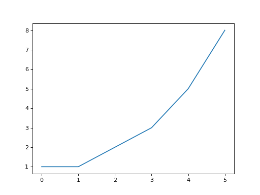
Matplotlib’s sphinx extension, which is included by the cookiecutter template, makes it possible to display matplotlib figures in line. This rst code:
.. plot::

   import matplotlib.pyplot as plt
   fig, ax = plt.subplots()
   ax.plot([1, 1, 2, 3, 5, 8])
renders in HTML as:
From here we refer you to the matplotlib plot directive documentation.
Math (LaTeX)
Sphinx can render LaTeX typeset math in the browser (using MathJax). This rst code:
.. math::

    \int_0^a x\,dx = \frac{1}{2}a^2
renders in HTML as:
This notation can also be used in docstrings. For example, we could add
the equation of Snell’s Law to the docstring of
snell().
Math can also be written inline. This rst code:
The value of :math:`\pi` is 3.141592653....
renders in HTML as:
The value of \(\pi\) is 3.141592653….
Referencing Documented Objects
You can create links to documented functions like so:
The :func:`example.refraction.snell` function encodes Snell's Law.
The example.refraction.snell() function encodes Snell’s Law.
Adding a ~ omits the module path from the link text.
The :func:`~example.refraction.snell` function encodes Snell's Law.
The snell() function encodes Snell’s Law.
See the Sphinx documentation for more.