Coulomb interactions

In this example we provide more details on how Coulomb interactions are implemented in multiplet calculations and EDRIXS in particular. We aim to clarify the form of the matrices, how they are parametrized, and how the breaking of spherical symmetry can switch on additional elements that one might not anticipate. Our example is based on a \(d\) atomic shell.

Create matrix

The Coulomb interaction between two particles can be written as

\[\begin{equation} \hat{H} = \frac{1}{2} \int d\mathbf{r} \int d\mathbf{r}^\prime \Sigma_{\sigma, \sigma^\prime} |\hat{\psi}^\sigma(\mathbf{r})|^2 \frac{e^2}{R} |\hat{\psi}^{\sigma^\prime}(\mathbf{r})|^2, \end{equation}\]

where \(\hat{\psi}^\sigma(\mathbf{r})\) is the electron wavefunction, with spin \(\sigma\), and \(R=|r-r^\prime|\) is the electron separation. Solving our problem in this form is difficult due to the need to symmeterize the wavefunction to follow fermionic statistics. Using second quantization, we can use operators to impose the required particle exchange statistics and write the equation in terms of a tensor \(U\)

\[\begin{equation} \hat{H} = \sum_{\alpha,\beta,\gamma,\delta,\sigma,\sigma^\prime} U_{\alpha\sigma,\beta\sigma^\prime,\gamma\sigma^\prime,\delta\sigma} \hat{f}^{\dagger}_{\alpha\sigma} \hat{f}^{\dagger}_{\beta\sigma^\prime} \hat{f}_{t\sigma^\prime}\hat{f}_{\delta\sigma}, \end{equation}\]

where \(\alpha\), \(\beta\), \(\gamma\), \(\delta\) are orbital indices and \(\hat{f}^{\dagger}\) (\(\hat{f}\)) are the creation (anihilation) operators. For a \(d\)-electron system, we have \(10\) distinct spin-orbitals (\(5\) orbitals each with \(2\) spins), which makes matrix the \(10\times10\times10\times10\) in total size. In EDRIXS the matrix can be created as follows:

import edrixs
import numpy as np
import scipy
import matplotlib.pyplot as plt
import itertools

F0, F2, F4 = 6.94, 14.7, 4.41
umat_chb = edrixs.get_umat_slater('d', F0, F2, F4)

We stored this under variable umat_chb where “cbh” stands for complex harmonic basis, which is the default basis in EDRIXS.

Parameterizing interactions

EDRIXS parameterizes the interactions in \(U\) via Slater integral parameters \(F^{k}\). These relate to integrals of various spherical Harmonics as well as Clebsch-Gordon coefficients, Gaunt coefficients, and Wigner 3J symbols. Textbooks such as [1] can be used for further reference. If you are interested in the details of how EDRIXS does this (and you probably aren’t) function umat_slater(), constructs the required matrix via Gaunt coeficents from get_gaunt(). Two alternative parameterizations are common. The first are the Racah parameters, which are

\[\begin{split}\begin{eqnarray} A &=& F^0 - \frac{49}{441} F^4 \\ B &=& \frac{1}{49}F^2 - \frac{5}{441}F^4 \\ C &=& \frac{35}{441}F^4. \end{eqnarray}\end{split}\]

or an alternative form for the Slater integrals

\[\begin{split}\begin{eqnarray} F_0 &=& F^0 \\ F_2 &=& \frac{1}{49}F^2 \\ F_4 &=& \frac{1}{441}F^4, \end{eqnarray}\end{split}\]

which involves different normalization parameters.

Basis transform

If we want to use the real harmonic basis, we can use a tensor transformation, which imposes the following orbital order \(3z^2-r^2, xz, yz, x^2-y^2, xy\), each of which involves \(\uparrow, \downarrow\) spin pairs. Let’s perform this transformation and store a list of these orbitals.

umat = edrixs.transform_utensor(umat_chb, edrixs.tmat_c2r('d', True))
orbitals = ['3z^2-r^2', 'xz', 'yz', 'x^2-y^2', 'xy']

Interactions

Tensor \(U\) is a series of matrix elements

\[\begin{equation} \langle\psi_{\gamma,\delta}^{\bar{\sigma},\bar{\sigma}^\prime} |\hat{H}| \psi_{\alpha,\beta}^{\sigma,\sigma^\prime}\rangle \end{equation}\]

the combination of which defines the energetic cost of pairwise electron-electron interactions between states \(\alpha,\sigma\) and \(\beta,\sigma^\prime\). In EDRIXS we follow the convention of summing over all orbital pairs. Some other texts count each pair of indices only once. The matrix elements here will consequently be half the magnitude of those in other references. We can express the interactions in terms of the orbitals involved. It is common to distinguish “direct Coulomb” and “exchange” interactions. The former come from electrons in the same orbital and the later involve swapping orbital labels for electrons. We will use \(U_0\) and \(J\) as a shorthand for distinguishing these.

Before we describe the different types of interactions, we note that since the Coulomb interaction is real, and due to the spin symmmetry properties of the process \(U\) always obeys

\[\begin{equation} U_{\alpha\sigma,\beta\sigma^\prime,\gamma\sigma^\prime,\delta\sigma} = U_{\beta\sigma,\alpha\sigma^\prime,\delta\sigma^\prime,\gamma\sigma} = U_{\delta\sigma,\gamma\sigma^\prime,\beta\sigma^\prime,\alpha\sigma} = U_{\gamma\sigma,\delta\sigma^\prime,\alpha\sigma^\prime,\beta\sigma}. \end{equation}\]

1. Intra orbital

The direct Coulomb energy cost to double-occupy an orbital comes from terms like \(U_{\alpha\sigma,\alpha\bar\sigma,\alpha\bar\sigma,\alpha\sigma}\). In this notation, we use \(\sigma^\prime\) to denote that the matrix element is summed over all pairs and \(\bar{\sigma}\) to denote sums over all opposite spin pairs. Due to rotational symmetry, all these elements are the same and equal to

\[\begin{split}\begin{eqnarray} U_0 &=& \frac{A}{2} + 2B + \frac{3C}{2}\\ &=& \frac{F_0}{2} + 2F_2 + 18F_4 \end{eqnarray}\end{split}\]

Let’s print these to demonstrate where these live in the array

for i in range(0, 5):
    val = umat[i*2, i*2 + 1, i*2 + 1, i*2].real
    print(f"{orbitals[i]:<8} \t {val:.3f}")

3z^2-r^2         4.250
xz               4.250
yz               4.250
x^2-y^2          4.250
xy               4.250

2. Inter orbital Coulomb interactions

Direct Coulomb repulsion between different orbitals depends on terms like \(U_{\alpha\sigma,\beta\sigma^\prime,\beta\sigma^\prime,\alpha\sigma}\). Expresions for these parameters are provided in column \(U\) in Table of 2 orbital interactions. We can print the values from umat like this:

for i, j in itertools.combinations(range(5), 2):
    val = umat[i*2, j*2 + 1, j*2 + 1, i*2].real
    print(f"{orbitals[i]:<8} \t {orbitals[j]:<8} \t {val:.3f}")

3z^2-r^2         xz              3.650
3z^2-r^2         yz              3.650
3z^2-r^2         x^2-y^2         2.900
3z^2-r^2         xy              2.900
xz               yz              3.150
xz               x^2-y^2         3.150
xz               xy              3.150
yz               x^2-y^2         3.150
yz               xy              3.150
x^2-y^2          xy              3.900

3. Inter-orbital exchange interactions

Exchange terms exist with the form \(U_{\alpha\sigma,\beta\sigma^\prime,\alpha\sigma^\prime,\beta\sigma}\). Expresions for these parameters are provided in column \(J\) of Table of 2 orbital interactions. These come from terms like this in the matrix:

for i, j in itertools.combinations(range(5), 2):
    val = umat[i*2, j*2 + 1, i*2 + 1, j*2].real
    print(f"{orbitals[i]:<8} \t {orbitals[j]:<8} \t {val:.3f}")

3z^2-r^2         xz              0.300
3z^2-r^2         yz              0.300
3z^2-r^2         x^2-y^2         0.675
3z^2-r^2         xy              0.675
xz               yz              0.550
xz               x^2-y^2         0.550
xz               xy              0.550
yz               x^2-y^2         0.550
yz               xy              0.550
x^2-y^2          xy              0.175

4. Pair hopping term

Terms that swap pairs of electrons exist as \((1-\delta_{\sigma\sigma'})U_{\alpha\sigma,\alpha\bar\sigma,\beta\bar\sigma,\beta\sigma}\) and depend on exchange interactions column \(J\) from Table of 2 orbital interactions and here in the matrix.

for i, j in itertools.combinations(range(5), 2):
    val = umat[i*2, i*2 + 1, j*2 + 1, j*2].real
    print(f"{orbitals[i]:<8} \t {orbitals[j]:<8} \t {val:.3f}")

3z^2-r^2         xz              0.300
3z^2-r^2         yz              0.300
3z^2-r^2         x^2-y^2         0.675
3z^2-r^2         xy              0.675
xz               yz              0.550
xz               x^2-y^2         0.550
xz               xy              0.550
yz               x^2-y^2         0.550
yz               xy              0.550
x^2-y^2          xy              0.175

5. Three orbital

Another set of terms that one might not immediately anticipate involve three orbitals like

\[\begin{split}\begin{equation} U_{\alpha\sigma, \gamma\sigma', \beta\sigma', \gamma\sigma} \\ U_{\alpha\sigma, \gamma\sigma', \gamma\sigma', \beta\sigma} \\ (1-\delta_{\sigma\sigma'}) U_{\alpha\sigma, \beta\sigma', \gamma\sigma', \gamma\sigma} \end{equation}\end{split}\]

for \(\alpha=3z^2-r^2, \beta=x^2-y^2, \gamma=xz/yz\). These are needed to maintain the rotational symmetry of the interations. See Table of 3 orbital interactions for the expressions. We can print some of these via:

ijkl = [[0, 1, 3, 1],
        [0, 2, 3, 2],
        [1, 0, 3, 1],
        [1, 1, 3, 0],
        [2, 0, 3, 2],
        [2, 2, 3, 0]]

for i, j, k, l in ijkl:
    val = umat[i*2, j*2 + 1, k*2 + 1, l*2].real
    print(f"{orbitals[i]:<8} \t {orbitals[j]:<8} \t"
          f"{orbitals[k]:<8} \t {orbitals[l]:<8} \t {val:.3f}")

3z^2-r^2         xz             x^2-y^2          xz              0.217
3z^2-r^2         yz             x^2-y^2          yz              -0.217
xz               3z^2-r^2       x^2-y^2          xz              -0.433
xz               xz             x^2-y^2          3z^2-r^2        0.217
yz               3z^2-r^2       x^2-y^2          yz              0.433
yz               yz             x^2-y^2          3z^2-r^2        -0.217

6. Four orbital

Futher multi-orbital terms include \(U_{\alpha\sigma,\beta\sigma^\prime,\gamma\sigma^\prime,\delta\sigma}\). We can find these here in the matrix:

ijkl = [[0, 1, 2, 4],
        [0, 1, 4, 2],
        [0, 2, 1, 4],
        [0, 2, 4, 1],
        [0, 4, 1, 2],
        [0, 4, 2, 1],
        [3, 1, 4, 2],
        [3, 2, 4, 1],
        [3, 4, 1, 2],
        [3, 4, 2, 1]]

for i, j, k, l in ijkl:
    val = umat[i*2, j*2 + 1, k*2 + 1, l*2].real
    print(f"{orbitals[i]:<8} \t {orbitals[j]:<8} \t {orbitals[k]:<8}"
          f"\t {orbitals[l]:<8} \t {val:.3f}")

3z^2-r^2         xz              yz              xy              -0.433
3z^2-r^2         xz              xy              yz              0.217
3z^2-r^2         yz              xz              xy              -0.433
3z^2-r^2         yz              xy              xz              0.217
3z^2-r^2         xy              xz              yz              0.217
3z^2-r^2         xy              yz              xz              0.217
x^2-y^2          xz              xy              yz              -0.375
x^2-y^2          yz              xy              xz              0.375
x^2-y^2          xy              xz              yz              -0.375
x^2-y^2          xy              yz              xz              0.375

Effects of multi-orbital terms

To test the effects of the multi-orbital terms, let’s plot the eigenenergy spectra with and without multi-orbital terms switched on for system with and without a cubic crystal field. We will use a \(d\)-shell with two electrons.

ten_dqs = [0, 2, 4, 12]

def diagonalize(ten_dq, umat):
    emat = edrixs.cb_op(edrixs.cf_cubic_d(ten_dq),
                        edrixs.tmat_c2r('d', ispin=True))
    H = (edrixs.build_opers(4, umat, basis)
         + edrixs.build_opers(2, emat, basis))
    e, v = scipy.linalg.eigh(H)
    return e - e.min()

basis = edrixs.get_fock_bin_by_N(10, 2)
umat_no_multiorbital = np.copy(umat)
B = F2/49 - 5*F4/441
for val in [np.sqrt(3)*B/2, np.sqrt(3)*B, 3*B/2]:
    umat_no_multiorbital[(np.abs(umat)- val) < 1e-6] = 0

fig, axs = plt.subplots(1, len(ten_dqs), figsize=(8, 3))

for cind, (ax, ten_dq) in enumerate(zip(axs, ten_dqs)):
    ax.hlines(diagonalize(ten_dq, umat), xmin=0, xmax=1,
              label='on', color=f'C{cind}')
    ax.hlines(diagonalize(ten_dq, umat_no_multiorbital),
              xmin=1.5, xmax=2.5,
              label='off',
              linestyle=':', color=f'C{cind}')
    ax.set_title(f"$10D_q={ten_dq}$")
    ax.set_ylim([-.5, 20])
    ax.set_xticks([])
    ax.legend()

fig.suptitle("Eigenvalues with 3&4-orbital effects on/off")
fig.subplots_adjust(wspace=.3)
axs[0].set_ylabel('Eigenvalues (eV)')
fig.subplots_adjust(top=.8)
plt.show()

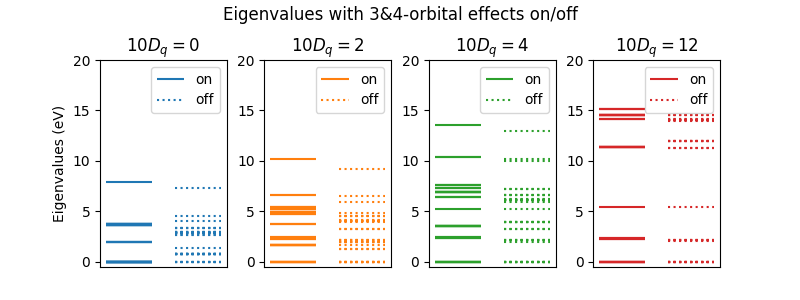
On the left of the plot Coulomb interactions in spherical symmetry cause substantial mxing between \(t_{2g}\) and \(e_{g}\) orbitals in the eigenstates and 3 & 4 orbital orbital terms are crucial for obtaining the the right eigenenergies. As \(10D_q\) get large, this mixing is switched off and the spectra start to become independent of whether the 3 & 4 orbital orbital terms are included or not.

Table of 2 orbital interactions

Orbitals \(\alpha,\beta\)	\(U_0\) Racah	\(U_0\) Slater	\(J\) Racah	\(J\) Slater
\(3z^2-r^2, xz\)	\(A/2+B+C/2\)	\(F_0/2+F_2-12F_4\)	\(B/2+C/2\)	\(F_2/2+15F_4\)
\(3z^2-r^2, yz\)	\(A/2+B+C/2\)	\(F_0/2+F_2-12F_4\)	\(B/2+C/2\)	\(F_2/2+15F_4\)
\(3z^2-r^2, x^2-y^2\)	\(A/2-2B+C/2\)	\(F_0/2-2F_2+3F_4\)	\(2B+C/2\)	\(2F_2+15F_4/2\)
\(3z^2-r^2, xy\)	\(A/2-2B+C/2\)	\(F_0/2-2F_2+3F_4\)	\(2B+C/2\)	\(2F_2+15F_4/2\)
\(xz, yz\)	\(A/2-B+C/2\)	\(F_0/2-F_2-12F_4\)	\(3B/2+C/2\)	\(3F_2/2+10F_4\)
\(xz, x^2-y^2\)	\(A/2-B+C/2\)	\(F_0/2-F_2-12F_4\)	\(3B/2+C/2\)	\(3F_2/2+10F_4\)
\(xz, xy\)	\(A/2-B+C/2\)	\(F_0/2-F_2-12F_4\)	\(3B/2+C/2\)	\(3F_2/2+10F_4\)
\(yz, x^2-y^2\)	\(A/2-B+C/2\)	\(F_0/2-F_2-12F_4\)	\(3B/2+C/2\)	\(3F_2/2+10F_4\)
\(yz, xy\)	\(A/2-B+C/2\)	\(F_0/2-F_2-12F_4\)	\(3B/2+C/2\)	\(3F_2/2+10F_4\)
\(x^2-y^2, xy\)	\(A/2+2B+C/2\)	\(F_0+4F_2-34F_4\)	\(C/2\)	\(35F_4/2\)

Table of 3 orbital interactions

Orbitals \(\alpha,\beta,\gamma,\delta\)		\(\langle\alpha\beta|\gamma\delta\rangle\) Racah	\(\langle\alpha\beta|\gamma\delta\rangle\) Slater
\(3z^2-r^2, xz, x^2-y^2, xz\)		\(\sqrt{3}B/2\)	\(\sqrt{3}F_2/2-5\sqrt{3}F_4/2\)
\(3z^2-r^2, yz, x^2-y^2, yz\)		\(-\sqrt{3}B/2\)	\(-\sqrt{3}F_2/2+5\sqrt{3}F_4/2\)
\(xz, 3z^2-r^2, x^2-y^2, xz\)		\(-\sqrt{3}B\)	\(-\sqrt{3}F_2+5\sqrt{3}F_4\)
\(xz, xz, x^2-y^2, 3z^2-r^2\)		\(\sqrt{3}B/2\)	\(\sqrt{3}F_2/2-5\sqrt{3}F_4/2\)
\(yz, 3z^2-r^2, x^2-y^2, yz\)		\(\sqrt{3}B\)	\(\sqrt{3}F_2-5\sqrt{3}F_4\)
\(yz, yz, x^2-y^2, 3z^2-r^2\)		\(-\sqrt{3}B/2\)	\(-\sqrt{3}F_2/2+5\sqrt{3}F_4/2\)

Table of 4 orbital interactions

Orbitals \(\alpha,\beta,\gamma,\delta\)		\(\langle\alpha\beta|\gamma\delta\rangle\) Racah	\(\langle\alpha\beta|\gamma\delta\rangle\) Slater
\(3z^2-r^2, xz, yz, xy\)		\(-\sqrt{3}B\)	\(-\sqrt{3}F_2+5\sqrt{3}F_4\)
\(3z^2-r^2, xz, xy, yz\)		\(\sqrt{3}B/2\)	\(\sqrt{3}F_2/2-5\sqrt{3}F_4/2\)
\(3z^2-r^2, yz, xz, xy\)		\(-\sqrt{3}B\)	\(-\sqrt{3}F_2+5\sqrt{3}F_4\)
\(3z^2-r^2, yz, xy, xz\)		\(\sqrt{3}B/2\)	\(\sqrt{3}F_2/2-5\sqrt{3}F_4/2\)
\(3z^2-r^2, xy, xz, yz\)		\(\sqrt{3}B/2\)	\(\sqrt{3}F_2/2-5\sqrt{3}F_4/2\)
\(3z^2-r^2, xy, yz, xz\)		\(\sqrt{3}B/2\)	\(\sqrt{3}F_2/2-5\sqrt{3}F_4/2\)
\(x^2-y^2 , xz, xy, yz\)		\(-3B/2\)	\(-3F_2/2+15F_4/2\)
\(x^2-y^2 , yz, xy, xz\)		\(3B/2\)	\(3F_2/2-15F_4/2\)
\(x^2-y^2 , xy, xz, yz\)		\(-3B/2\)	\(-3F_2/2+15F_4/2\)
\(x^2-y^2 , xy, yz, xz\)		\(3B/2\)	\(3F_2/2-15F_4/2\)

Footnotes

[1]

MSugano S, Tanabe Y and Kamimura H. 1970. Multiplets of Transition-Metal Ions in Crystals. Academic Press, New York and London.